我将2017冬季与2018秋季Stanford的CS 106X作业发布在我的Github仓库.
CS 106X Lecture 2 – Functions & Strings
Output Parameters
Pass by reference to return multiple items.
当pass by value时,参数会复制一份到函数自身的frame里,所以外部的值不会改变,但是pass by reference是传指针。
当我们通过传递指针的方式像函数传递参数时,程序会将原本的指针复制一份到函数栈中,新复制的指针与主函数中的指针指向相同的地址,这意味着我们可以修改指针指向的对象,但是如果我们修改指针本身,那么主函数中的指针不会被影响。这意味着在某些操作,比如如果我们想要向二叉树中插入节点,或者删除二叉树中的某个节点时,我们要传递引用,因为这些操作牵扯到了修改指针本身。而如果我们仅仅是想要修改指针指向的对象,比如传入一个指向数组的指针,修改数组的值,那么此时不需要传递引用。
void datingRange(int age, int& min, int& max) {
    min = age / 2 + 7; max = (age - 7) * 2;
}
int main() {
    int young;
    int old;
    datingRange(48, young, old);
    cout << "A 48-year-old could date someone from " << young << " to " << old " years old." << endl;
}
Default Parameters
All parameters with default value must appear last in the formals list.
C String bugs
C本身提供的字符串不具备+,find等一系列功能,所以在使用时,最好要转化为C++格式的字符串,用string类型做变量类型声明:
string("text") C string to C++ string –
string.c_str() C++ string to C string
string s = string("hi") + "there";
string s = "hi";           // convert to C++ string (auto-conversion)

s += "there";
CS 106X Lecture 3 – Vectors & Grid; IO stream
Vector & Grid
使用方法:
Vector<int> names;
names.add("Dog");

Grid<int> matrix(3,4);
可以使用range for loop:
for(int value: matrix){
    // do something with value;
}
// "for-each" by  reference

for (string& name: names){
    name += "!";
}
当他们作为函数参数使用时,要注意传递引用,
pass by value是很慢的
Remove?
当我们试图从Vector中删除元素时,最好的遍历方法是自后向前遍历,这样可以避免因为删除元素带来的shifting的影响。
IO Stream
- 整行读取
iftream input;
input.open("poem.txt");
if (input.fail()){
    // do something if fails;
}
else{
    string line;
    while(getline(input, line)){
    cout << line << endl;
	}
}
input.close();
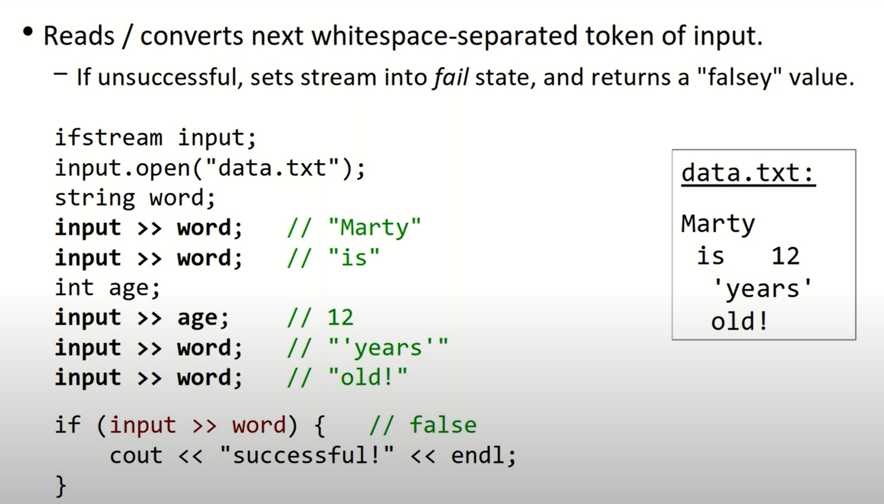
- 单词读取
ifstream file;
file.open(filename);
string word;

while(input >> word){
    // do something with words
}
一种错误的文件遍历方法:
while(!input.fail()){
    string line;
    getline(input, line);
    cout << line << endl;
}
这种方法的问题在于,会多遍历一行(可能是空行),因为在读取完最后一行的数据后,input.fail仍然为false.
我们也可以通过操作符>>进行文件读取:
- tokenize a string
使用<sstream>:
istringstream input("test string 12345");
string first, last;
int phone;
input >> first >> last; // first = "test", last = "string"

input >> phone; // 12345
同样地,我们也可以使用之前的while循环来读取所有tokens。
- write output to a string buffer (without display directly)
int age = 42, iq = 45;
ostringstream output;
output << "Zoidberg's age is " << age << endl;
output << "and his IQ is " << iq << "!" << endl;

// use the str method to extract the string that was built

string result = output.str();
CS 106X HW1 - Game Of Life
遇到的一个问题:
当我试图使用pass by value的方式将ifstream file传入函数参数时,程序报错:deleted copy constructor.
在查阅了《C++ Primer》中有关于拷贝构造函数的相关内容(P449)后,发现这是由于某些类(比如ifstream),也包括<iostream>在定义类时阻止了拷贝,以避免多个对象写入或者读取相同的IO缓冲。在新标准下,将拷贝构造函数和拷贝赋值运算符定义为删除的函数来阻止拷贝。在函数的参数列表后边加上=delete来指出我们希望将它定义为删除的,所以在pass by value时,因为要调用相关类的拷贝构造函数,就会被阻止操作。
我们可以通过pass by reference或者直接将文件操作流定义为引用对象来解决这一问题。

CS 106X Lecture 4 – Stacks & Queues
Stack
课堂上一个有趣的例子:关于使用stack进行括号匹配判断:
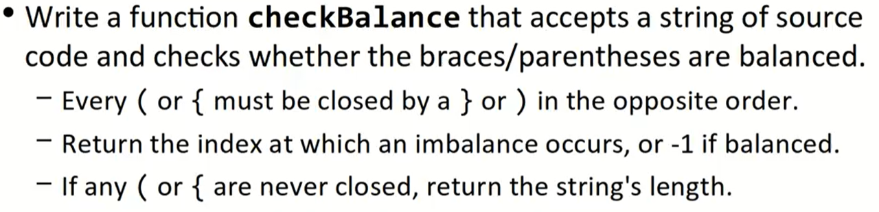
int checkBalance(string code){
    Stack<char> stack_code;
    for(int i = 0; i < code.length(); ++i){
        if (code[i] == "(" || code[i] == "{") stack_code.push(code[i]);

        else if (code[i] == ")" || code[i] == "}") stack_code.pop()
    }
    return -1;
}
这样的弹出代码是不对的,必须在栈顶检测到匹配的括号类型时,才将其弹出,如果此时栈顶括号类型不匹配,说明这段字符串本身的括号就是不匹配的。同时,考虑到可能出现只有左括号而永远没有闭合的情况,这段代码应做如下修改:
int checkBalance(string code){
    Stack<char> stack_code;
    for(int i = 0; i < code.length(); ++i){
        if (code[i] == "(" || code[i] == "{") stack_code.push(code[i]);
        else if (code[i] == ")" ) {
            if (stack_code.peek() == "(") stack_code.pop();
            else return i;
        }
        else if (code[i] == "}") {
            if (stack_code.peek() == "{") stack_code.pop();
            else return i;
        }
    }
    if (!stack_code.isEmpty()) return code.length;
    return -1;
}
Queue
一个mirror问题:queue: {a, b, c} -> {a, b, c, c, b, a}
void mirror(Queue<string>& queue){
    Stack<string> mirror_stack;
    while (!queue.isEmpty()){
        string s = queue.dequeue();
        mirror_stack.push(s);
    }
    // q = {}

    // mirror_stack = {a, b, c} top
}
但现在的问题在于想要保存原来的序列,所以考虑在对队列dequeue的同时,把数据保存进这个队列(基于FIFO的特性):
void mirror(Queue<string>& queue){
    Stack<string> mirror_stack;
    Stack<string> mirror_stack;
    // 改为for循环

    for (int i = 0; i < queue.length(); ++i){
        string s = queue.dequeue();
        mirror_stack.push(s);
        // 加入queue

        queue.enqueue(s);
    }
    // q = {a, b, c} back

    // mirror_stack = {a, b, c} top

    while (!stack.isEmpty()){
        queue.enqueue(stack.pop());
    }
}
CS 106X Lecture 5 – Set & Maps
Set
Perform add/remove/search(contains) efficientlyNo indexes
| Sorted or not | search speed | implementation | |
|---|---|---|---|
| Set | Sorted order | fast | binary tree |
| HashSet | unpredictable order | pretty fast | hash table |
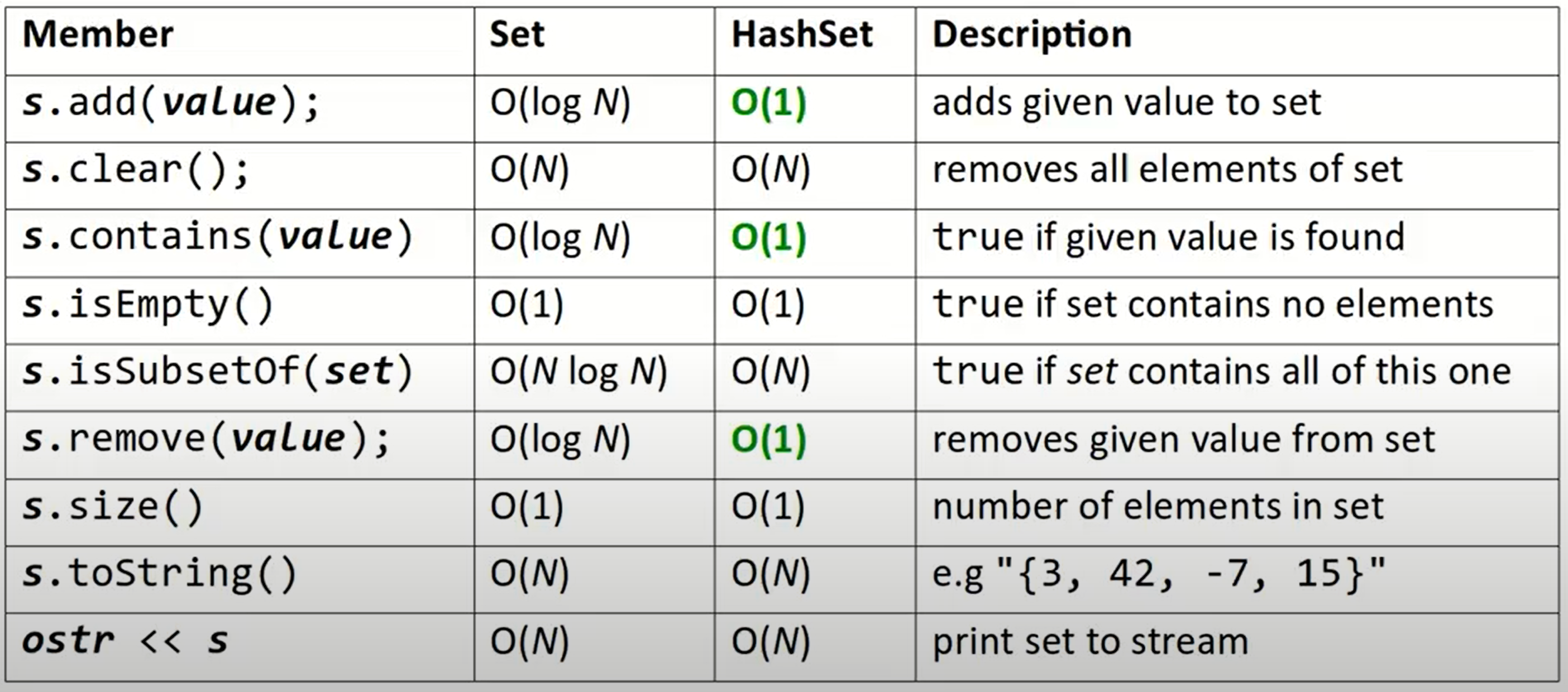
Set可以理解为一个集合,可以进行与string类类似的操作。
遍历方法:
for (type name: collection){
    statements;
}
如果定义了自己的struct或者class,是不能直接多次加入set的,我们需要对
<进行运算符重载
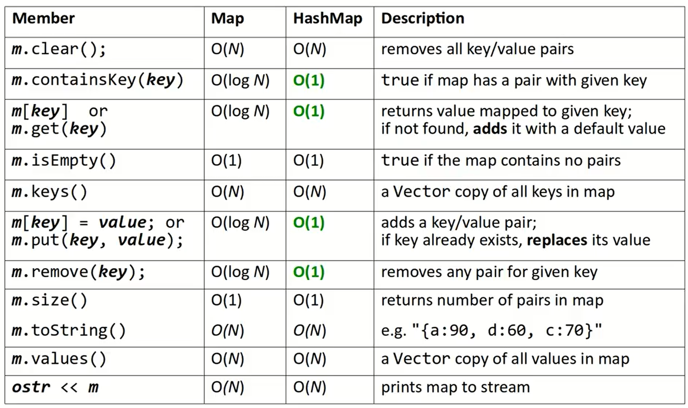
Maps
类似于Python的字典,储存的是Pair
类型类似于Set
CS 106X Lecutre 7-9 Basic Recursion
这里记录老师上课的几个例子,比较典型的说明了可以对需要进行递归的函数添加的辅助操作:
Crawl file / directory
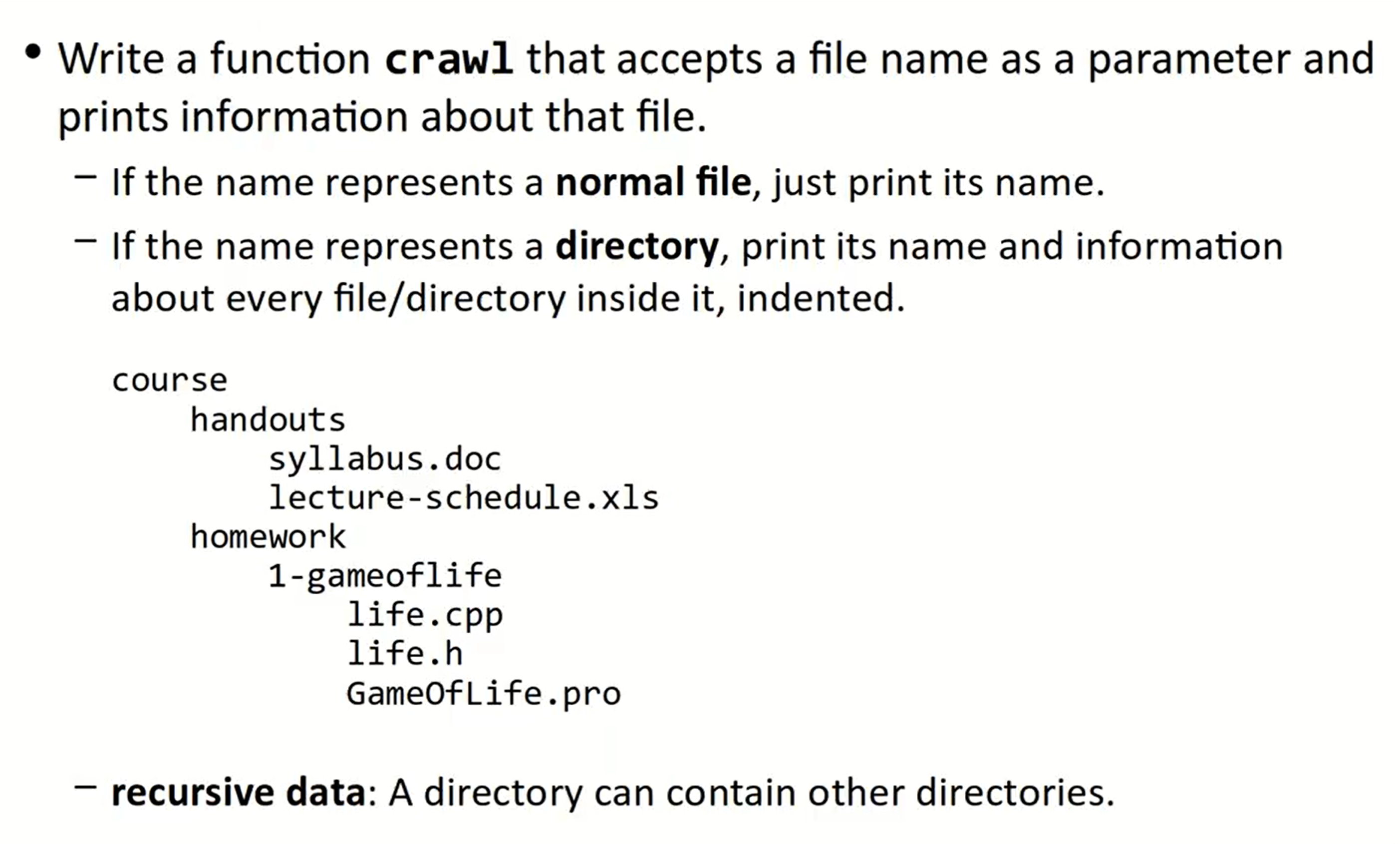
void crawl(const string& filename) {
    // both of the two cases need to be printed

    // cout << filename << endl;

    cout << getTail(filename) << endl;
    if(isFile(filename)) {
        // base case: normal file

    }
    else {
        // recursive case: directory

        Vector<string> files = listDirectory(filename);
        for (string &file: files) {
            // crawl(file);

            crawl(filename + "/" + file);
        }
    }
}
到了这一步,我们来补齐每个句子前边的缩进,通过在函数参数中添加默认参数实现对递归中缩进的递增,通过在for循环中递增缩进参数来实现递增:
void crawl(const string& filename, string indent = "") {
    cout << indent << getTail(filename) << endl;
    if(isFile(filename)) {
        // base case: normal file

    }
    else {
        // recursive case: directory

        Vector<string> files = listDirectory(filename);
        for (string &file: files) {
            // cout << "    " + indent;

            crawl(filename + "/" + file, indent + "    ");
        }
    }
}
Evaluate
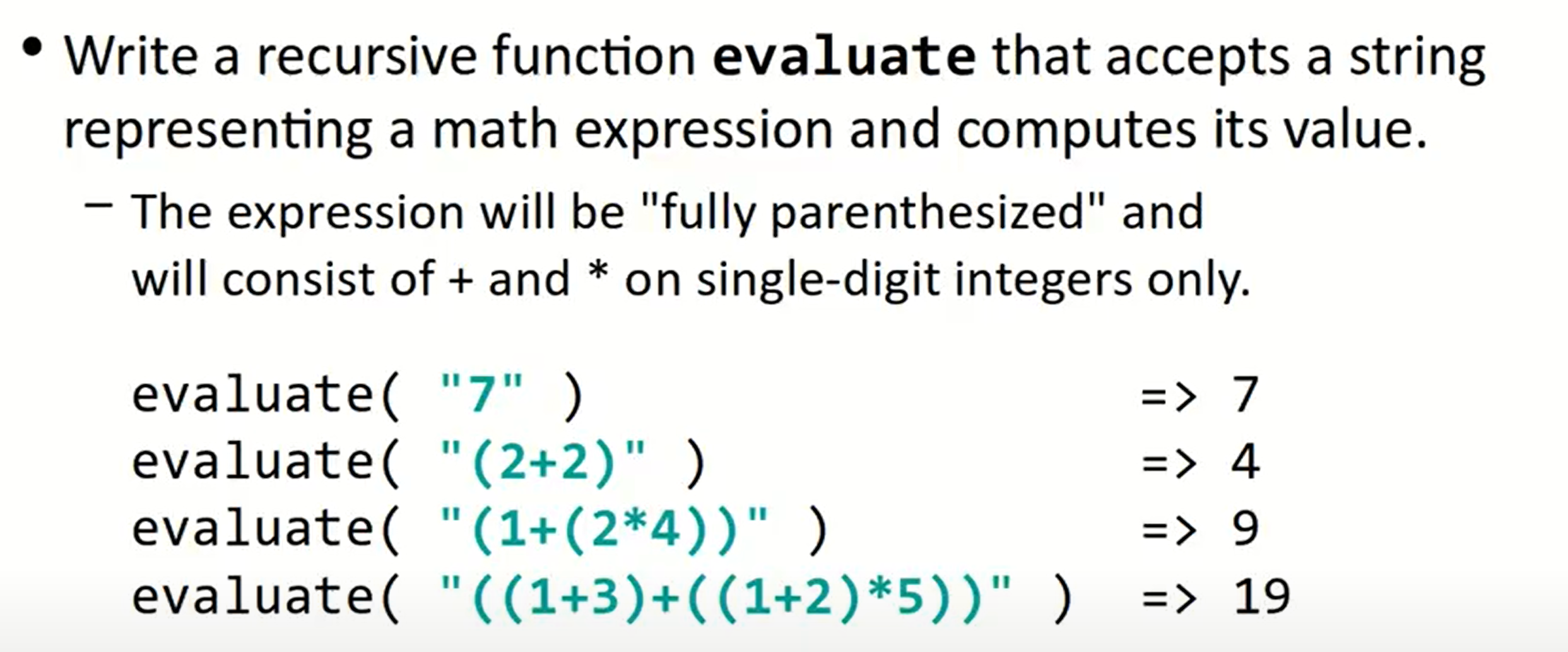
注意这道题本身带有很多的限制条件,我们可以利用这些限制条件写出一个比较简单的递归函数,而不用借助多次复杂的数据结构;所以我们尝试增加一个变量,跟中遍历字符串位置:
int evaluate(const string & exp) {
    int index = 0;
    return evaluate_helper(exp, index);
}

int evaluate_helper(const string & exp, int index) {
    // base case

    if(isdigit(exp[index])) {
        // transform from the char to int

        int result = exp[index] - '0';
        index++;
        return result;
    }
    // recursive case

    else {

    }
}
在思考recursive case的时候,我们要想在这个问题中,什么才是self-similar problem,很明显每一对括号都是一个self-similar problem,所以在遇到这些self-similar problem的时候,进行递归。
int evaluate(const string & exp) {
    int index = 0;
    return evaluate_helper(exp, index);
}

int evaluate_helper(const string & exp, int index) {
    if(isdigit(exp[index])) {
        int result = exp[index] - '0';
        index++;
        return result;
    }
    // recursive case

    else {
        // this "if" can be deleted, since it is the only other case

        if (exp[index] == '(') {
            // skip '('

            index++;
            // operand->operator->operand

            // assume this function will return what we want:

            int left = evaluate_helper(exp, index);
            char operand = exp[index];
            index++;
            int right = evaluate_helper(exp, index);
            if (operand == '+') {
                return left + right;
            }
            if (operand == '*') {
                return left * right;
            }
            // skip ')'

            index++;
        }
        // ')'

        // +, *
    }
}
CS 106X Lecture 10-12 Exhaustive Search & Backtrack
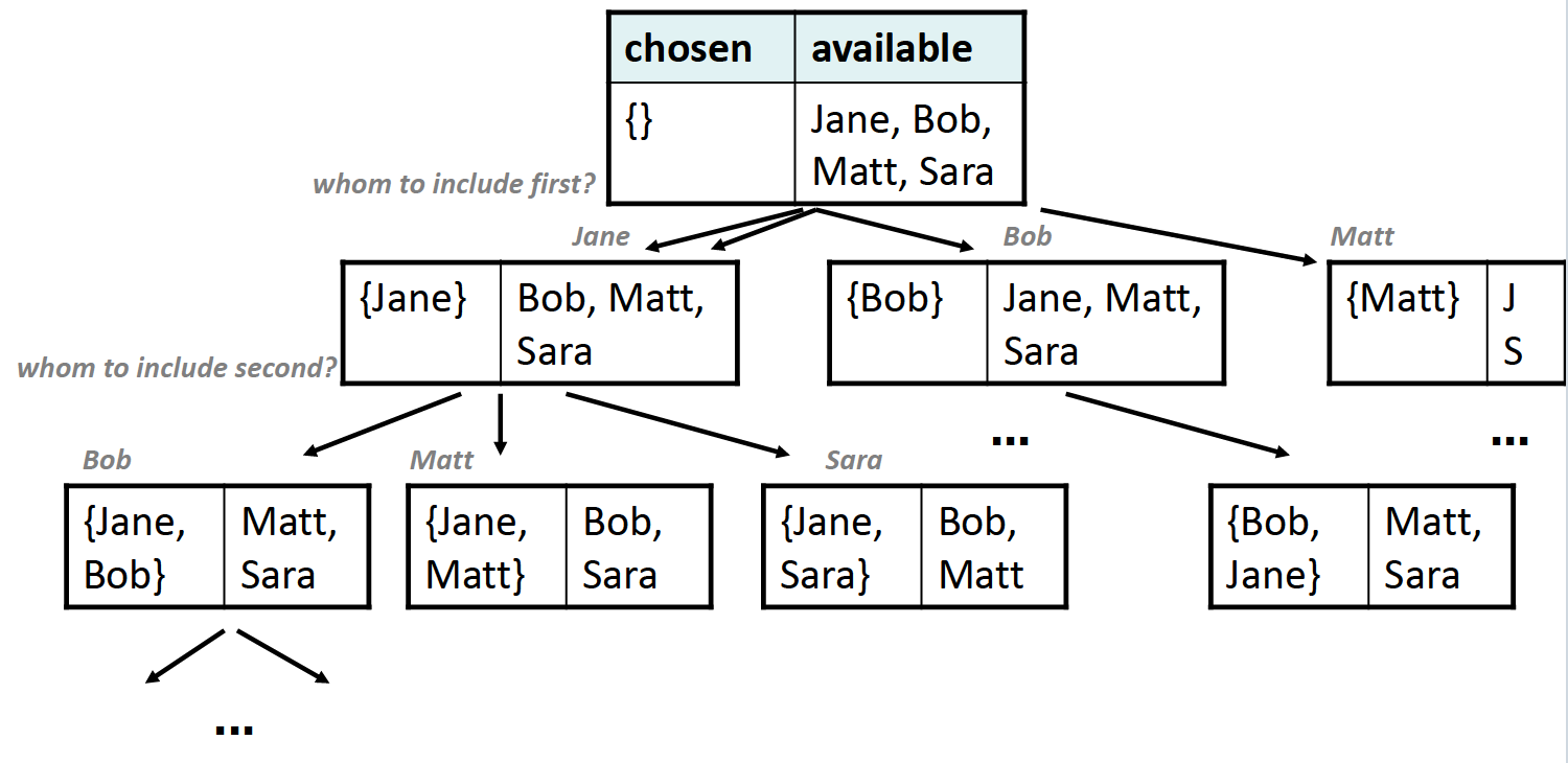
Exhaustive Search
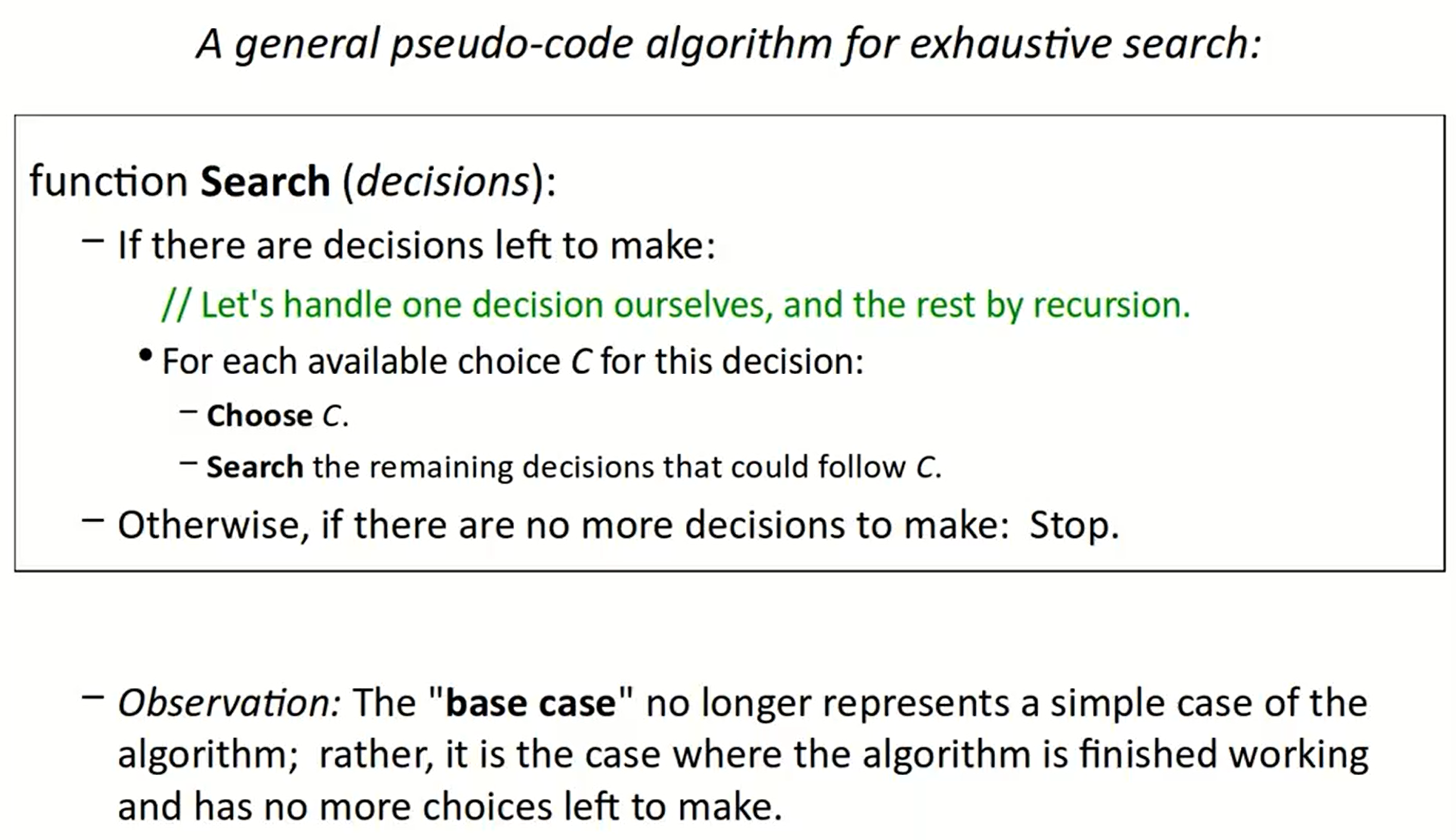
使用递归实现穷举搜索的方法类似于CS 61A中的tree recursion,在某一时间节点,我们有两种(或者多种选择),每一种选择又对应着一个与原问题self-similar的递归问题。
特别的是,在这种问题里,base case更恰当的理解方式是已经没有多余选择。
课堂上的几个例子比较具有代表性,在这里予以记录:
PrintBinary
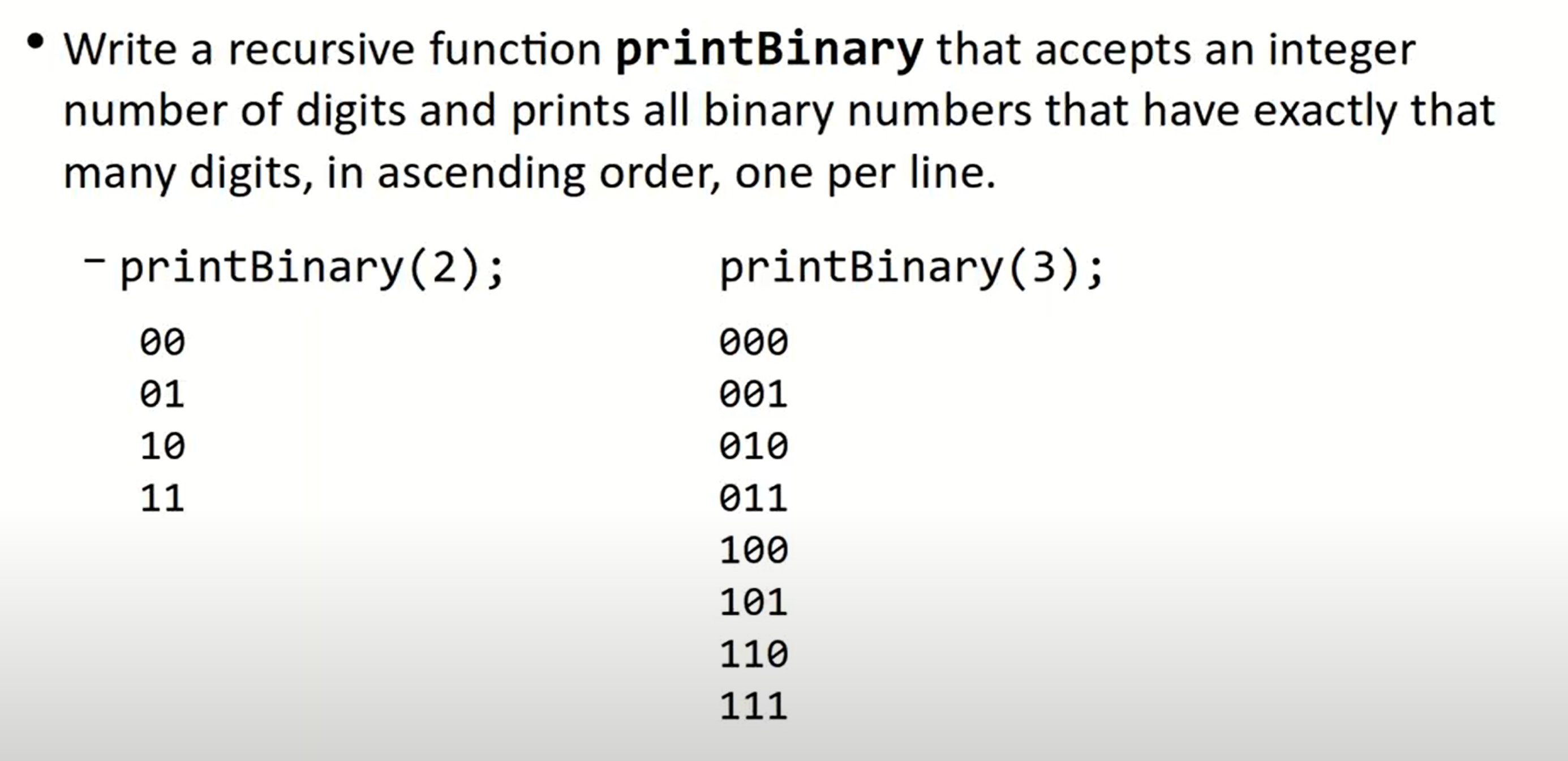
printBinary(3)第一次选择(0/1)后,问题便转化为printBinary(2),所以问题的基本框架是:
void printBinary(int digits) {
    if (digits == 0) {
        // there is no more choice

    }
    else {
        // do something to indicate using 0
        printBinary(digits - 1);
        // do something to indicate using 1
        printBinary(digits - 1);
    }
}
为了能够保存到底使用了0还是1的这种数据,我们对函数做出如下改变:
void printBinary(int digits, string prefix) {
    if (digits == 0) {
        // there is no more choice
        cout << prefix << endl;
    }
    else {
        // do something to indicate using 0
        printBinary(digits - 1, prefix + "0");
        // do something to indicate using 1
        printBinary(digits - 1, prefix + "1");
    }
}
正如在CS 61A中的描述的tree recursion一样,最终的调用树如下:
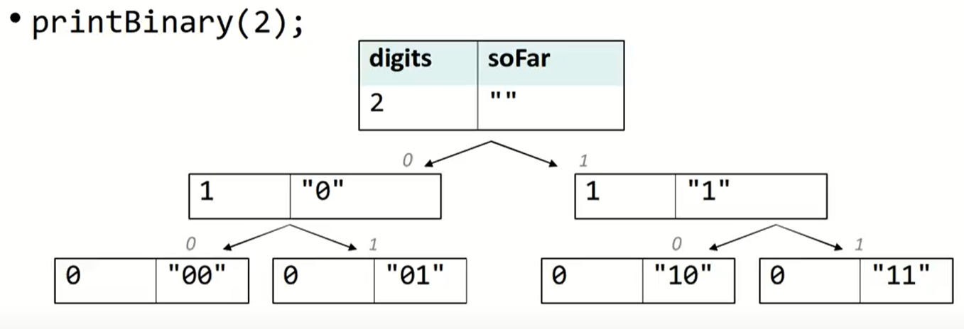
这种树被称为call tree或者decision tree.
如果将此题中的二进制数字改为十进制数字,那么最好借助于for循环规范代码(也与CS 61A中教授的方法相同):
void printDecimal(int digits, string prefix) {
    if (digits == 0) {
        cout << prefix << endl;
    }
    else {
        for (int i = 0; i <= 9; ++i) {
            printDecimal(digits - 1, prefix + integerToString(i));
        }
    }
}
Permutations
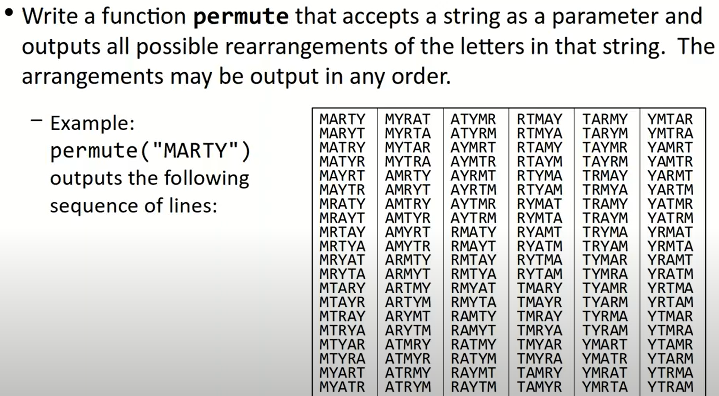
void permute(string s, string prefix) {
    if (s == "") {
        cout << prefix << endl;
    }
    else {
        // 每一个字母都可以作为第一个字母出现
        for (int i = 0; i < s.length(); ++i) {
            char cur = s[i];
            // 将选定的字母从序列中去除,之后不再出现
            str = s.substr(0, i) + s.substr(i + 1);
            permute(str, prefix + cur);
        }
    }
}
如果我们想把所有的结果保存起来,则需要借助数据结构和一个helper函数:
Vector<string> permute(string s) {
    Vector<string>& v;
    permuteHelper(s, "", v);
    return v;
}

void permute(string s, string prefix, Vector<string>& v) {
    if (s == "") {
        // cout << prefix << endl;
        v.add(prefix);
    }
    else {
        // 每一个字母都可以作为第一个字母出现
        for (int i = 0; i < s.length(); ++i) {
            char cur = s[i];
            // 将选定的字母从序列中去除,之后不再出现
            str = s.substr(0, i) + s.substr(i + 1);
            permute(str, prefix + cur);
        }
    }
}
Backtracking
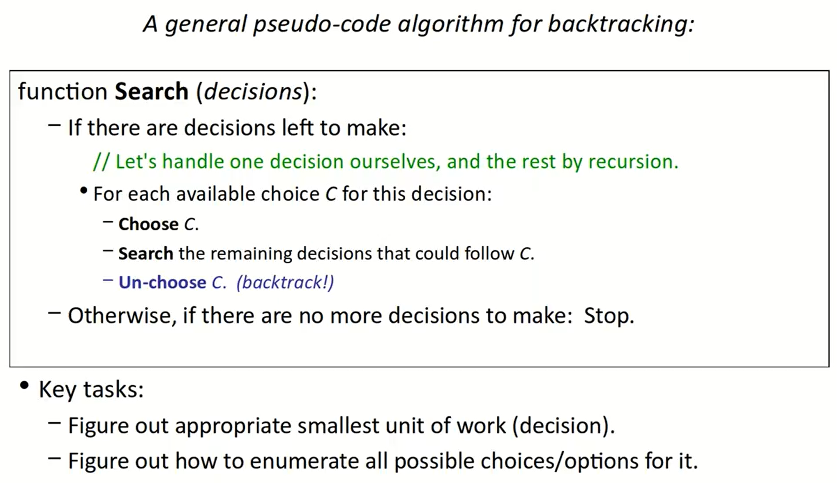
与穷举所不同的是,在回溯问题中,因为在递归之后可能改变了原本数据的组成结构和状态,所以我们要进行un-choose。或者说我们可能会遇到某些情况,导致需要舍弃掉当前的选择,并回退到上一步重新进行选择。
回溯算法一般分为三步:
- choose
- explore
- un-choose
Dice rolls
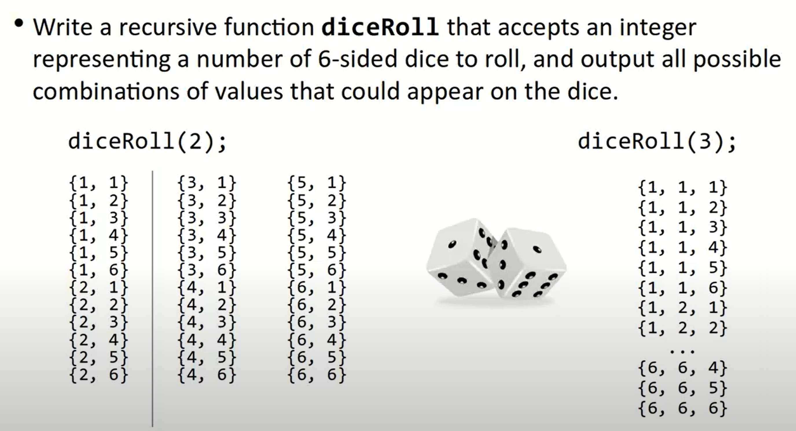
Vector<int> diceRolls(int dice) {
    Vector<int> v;
    diceHelper(dice, v);
    return v;
}

void diceHelper(int dice, Vector<int> & chosen) {
    if (dice == 0) {
        cout << chosen << endl;
    }
    else {
        for (int i = 1; i <= 6; ++i) {
        	// choose
            chosen.add(i);
            // search/explore
            diceHelper(dice - 1, chosen);
            // un-choose
            chosen.remove(chosen.size() - 1);
        }
    }
}
为什么这里需要un-choose的步骤?
因为我们需要储存的是每一种单独的选择组合,在
explore的过程中,我们改变了chosen中的数据存储,如果不进行un-choose的步骤,那么chosen的数据会一直保存下来。而在这里,un-choose的步骤刚好能够去除在每一次运行中添加在chosen中的元素。
为什么在exhaustive search中的permutations不需要un-choose的步骤?
因为在那道题目中,
prefix不是按引用传递的,而在这道题目中,vector按照引用传递。
Dice roll sum
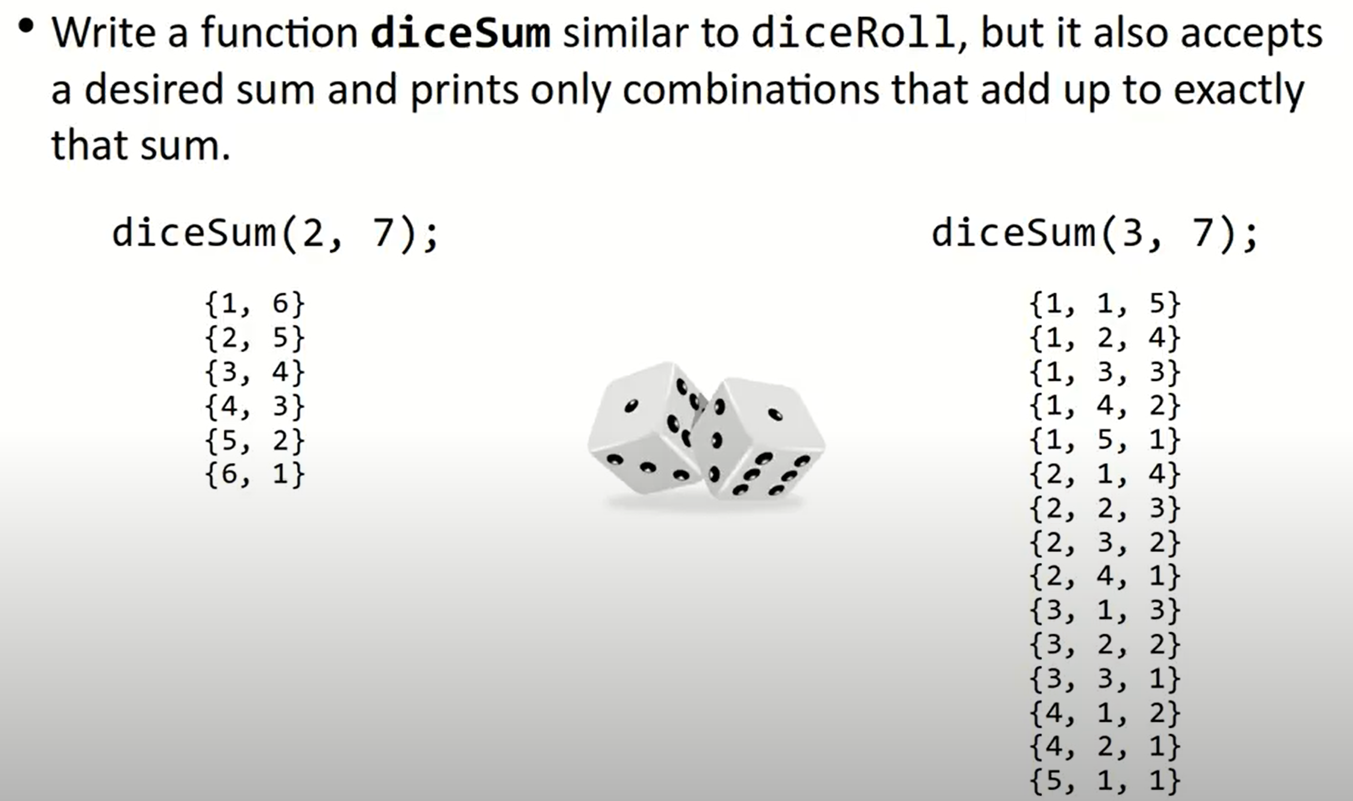
这道题目比较容易能想到使用回溯法做了:
Vector<int> diceSum(int dice) {
    Vector<int> v;
    diceHelper(dice, v);
    return v;
}

void diceSumHelper(int dice, int desiredSum, Vector<int> & chosen) {
    // if there is no choice to make
    if (dice == 0) {
        if (sumAll(chosen) == desiredSum) {
            cout << chosen << endl;
        }
    }
    else {
        for (int i = 1; i <= 6; ++i) {
        	// choose
            chosen.add(i);
            // search/explore
            diceHelper(dice - 1, desiredSum, chosen);
            // un-choose
            chosen.remove(chosen.size() - 1);
        }
    }
}
但是这个解法中毫无疑问经过了多次没有必要的函数运行,因为我们先是计算出了所有的可能的组合,之后只把符合条件的输出了,而我们本可以直接根据和的情况舍弃一些值,不继续进行函数循环:
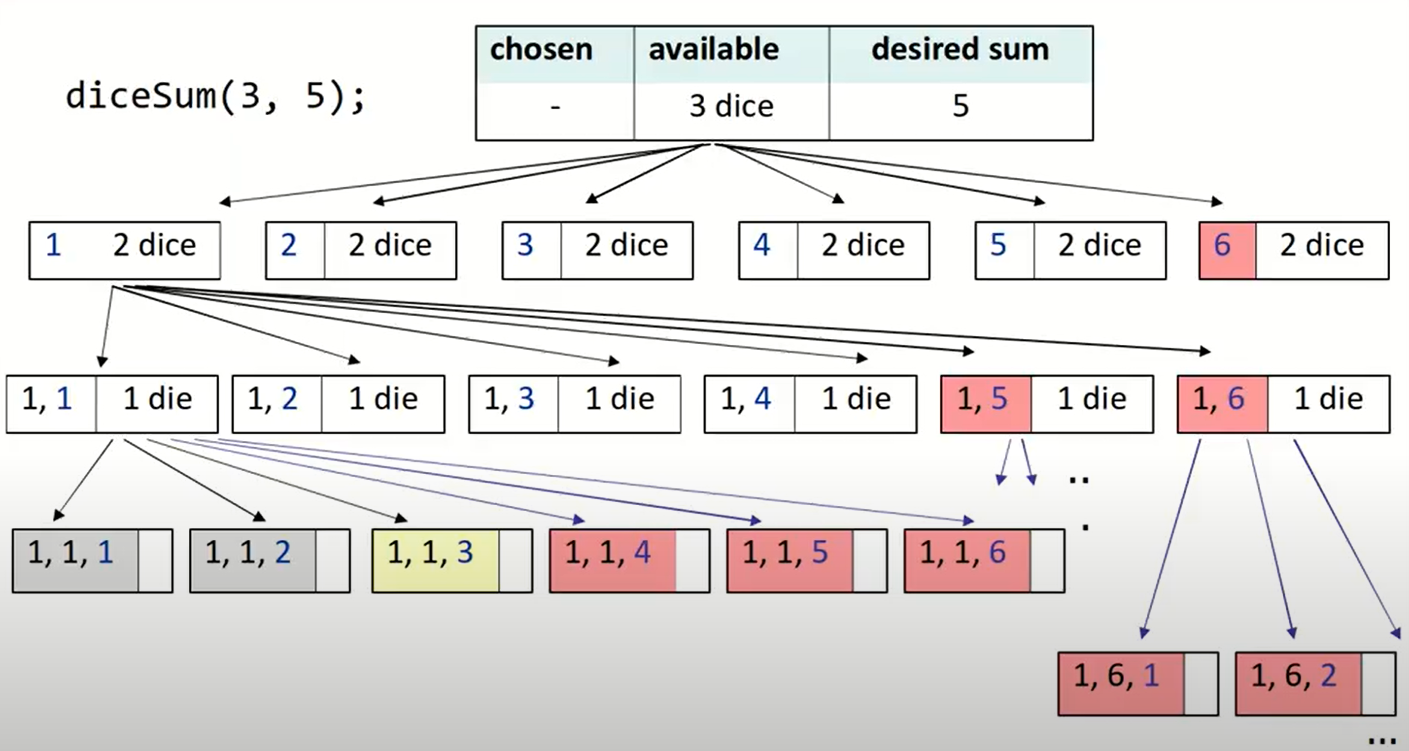
(红色标注的均是可以舍弃的情况)
所以这里就用到了回溯算法中经常结合的一个操作:剪枝操作。
- computing sum over and over is wasteful
- don’t explore decision trees where values are too low/high
Vector<int> diceSum(int dice) {
    Vector<int> v;
    diceSumHelper(dice, 0, v);
    return v;
}

void diceSumHelper(int dice, int desiredSum, Vector<int> & chosen) {
    // if there is no choice to make
    if (dice == 0) {
        if (desiredSum == 0) {
            cout << chosen << endl;
        }
    }
    else {
        for (int i = 1; i <= 6; ++i) {
            int max = desiredSum - i - 1 * (dice - 1);
            int min = desiredSum - i - 6 * (dice - 1);
            if (max >= 0 && min <= 0) {
                // choose
                chosen.add(i);
                // search/explore
                diceHelper(dice - 1, desiredSum - i, chosen);
                // un-choose
                chosen.remove(chosen.size() - 1);
            }
        }
    }
}
如果我们再对此题进行改编:
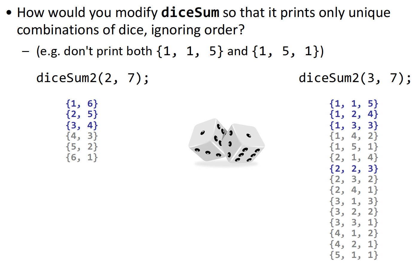
可以想到,我们需要一个参数来保存前一个只,并保证当前要选择的值必须不小于前一个值,之后将该参数更新为此次选择的值:
Vector<int> diceSum(int dice) {
    Vector<int> v;
    diceSumHelper(dice, 0, v, 0);
    return v;
}

void diceSumHelper(int dice, int desiredSum, Vector<int> & chosen, int curMinValue) {
    // if there is no choice to make
    if (dice == 0) {
        if (desiredSum == 0) {
            cout << chosen << endl;
        }
    }
    else {
        // update the for iteration
        for (int i = curMinValue; i <= 6; ++i) {
            // also update this formula
            int max = desiredSum - i - i * (dice - 1);
            int min = desiredSum - i - 6 * (dice - 1);
            if (max >= 0 && min <= 0) {
                // choose
                chosen.add(i);
                // search/explore
                diceHelper(dice - 1, desiredSum - i, chosen, i);
                // un-choose
                chosen.remove(chosen.size() - 1);
            }
        }
    }
}
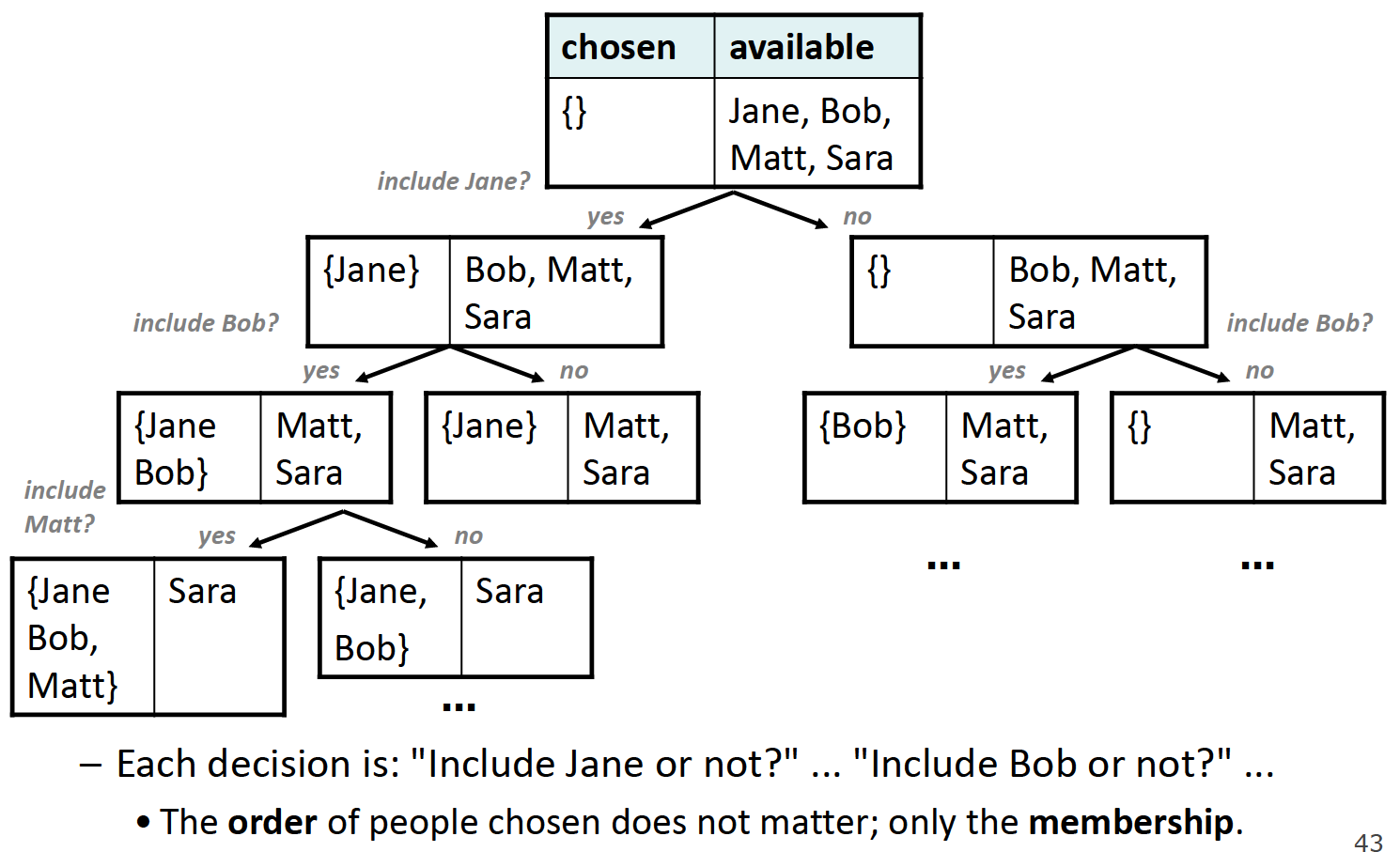
Subsets
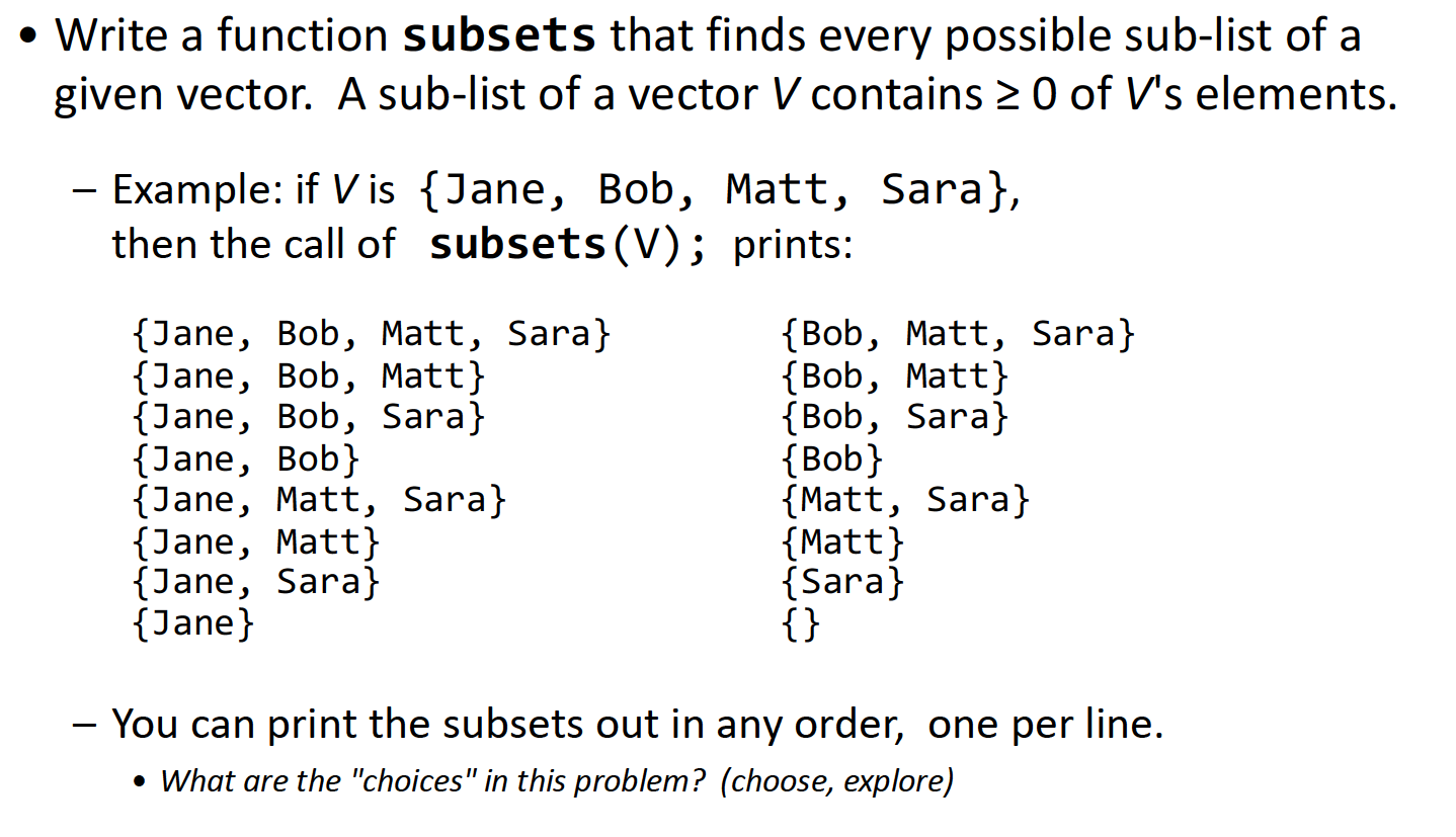
这道题很容易出现的错误是vector中元素顺序不一样,但是含有的元素是一样的,即下图所示:
为了避免这种情况的出现,我们应该把做选择的依据变更为:是否包含某个元素,而非先包含哪个元素。所以这道题目里不应当使用for循环,否则会造成重复选择,正确的decision tree如下:
Vector<string> subsets(Vector<string>& v) {
    Vector<string> chosen;
    sublistHelper(v, chosen);
    return chosen;
}

void sublistHelper(Vector<string>& v, Vector<string>& chosen) {
    if (v.isEmpty()) {
        cout << chosen << endl;
    }
    else {
        // choose
        string mine = v[0];
        v.remove(0);
        // explore/search

        // Yes, include them
        chosen.add(mine);
        sublistHelper(v, chosen);
        // No, exclude them
        chosen.remove(chosen.size() - 1);
        subslitHelper(v, chosen);

        // un-choose
        v.insert(0, mine);
    }
}
8 Queens Problem
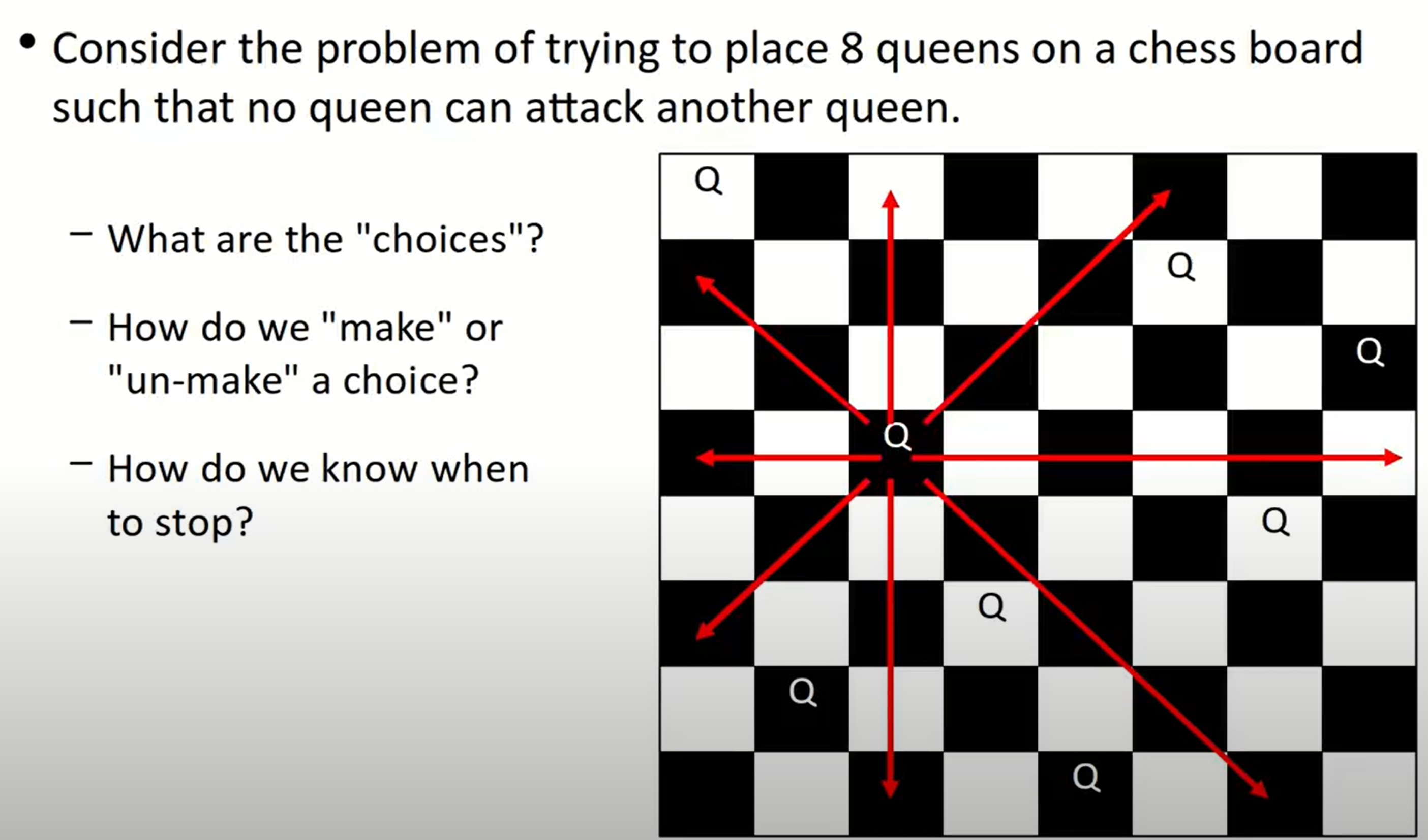
一个比较简单的出发点是观察到在每一行以及每一列,一定存在并且仅存在一个queen。考虑每一行(或者每一列),然后对其中的每一列(每一行)的点逐个判定是否是可以摆放的点(是否安全),整体上使用回溯法解决:如果当前行(列)满足条件(可以摆放),那么就继续探索(坐标移到下一行(列)),否则将板上的皇后去掉:
void solveQueensHelper(Board& board, int col) {
    if (col >= board.size()) {
        // base case
        cout << board << endl;
    }
    else {
        for (int row = 0; row < board.size(); ++row) {
            if (board.isSafe(row, col)) {
                // choose
                board.place(row, col);
                // explore
                solveQueensHelper(board, col + 1);
                // un-choose
                board.remove(row, col);
            }
        }
    }
}
如果我们想让程序仅输出一个正确结果:
bool solveQueensHelper(Board& board, int col) {
    if (col >= board.size()) {
        // base case
        cout << board << endl;
        return true;
    }
    else {
        for (int row = 0; row < board.size(); ++row) {
            if (board.isSafe(row, col)) {
                // choose
                board.place(row, col);
                // explore
                bool result = solveQueensHelper(board, col + 1);
                if (result) {
                    return true;
                }
                // un-choose
                board.remove(row, col);
            }
        }
        return false;
    }
}
Travel
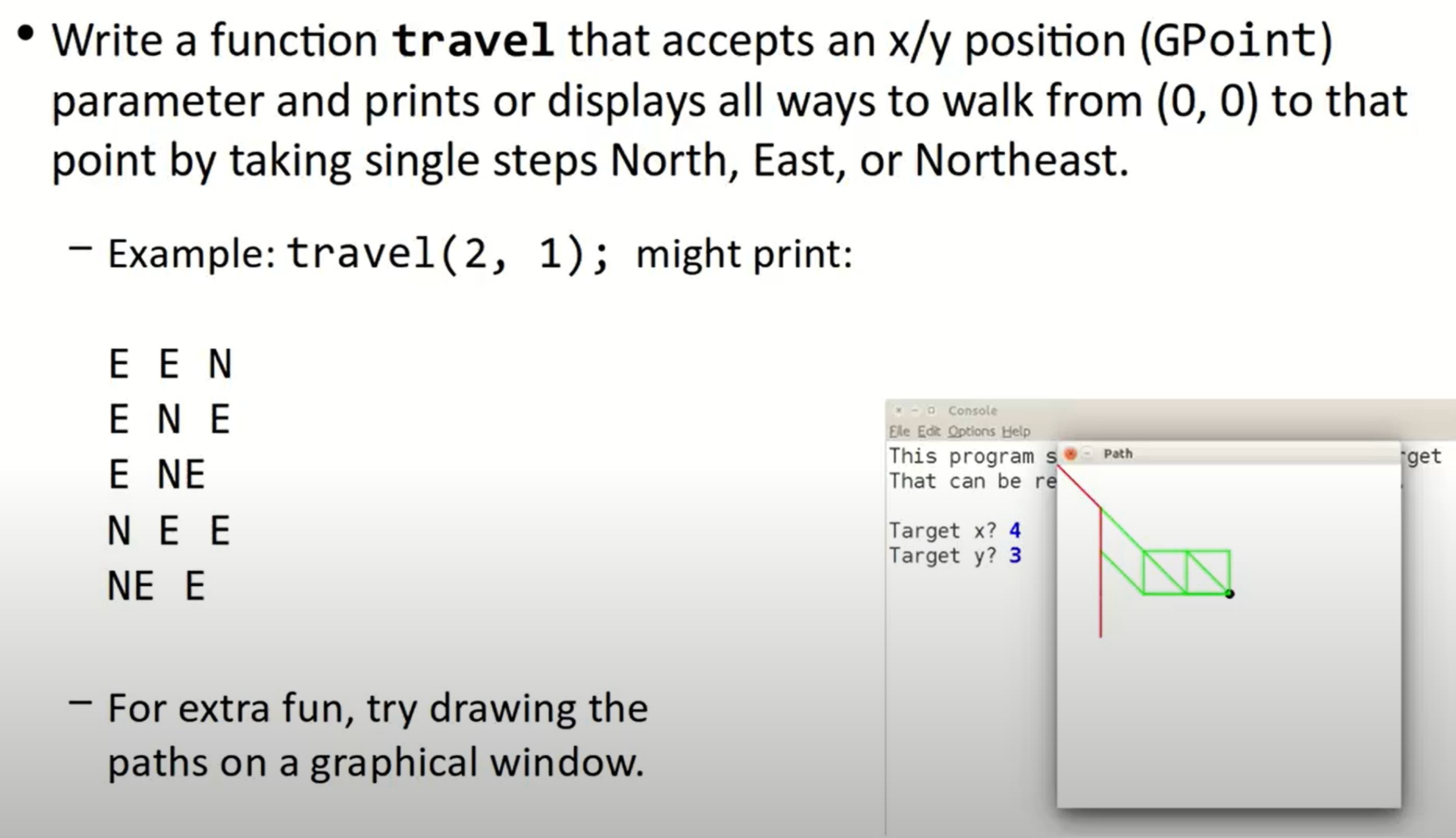
这也是一个backtracking的问题,因为在穷举搜索的基础上,会存在一些bad case使得我们无法到达目标指定位置,那我们需要回溯到上一步的位置:
Vector<string> travel(const GPoint & target) {
    GPoint origin(0, 0);
    Vector<string> path;
    travelHelper(target, origin, path);
    return path;
}

void travelHelper(const GPoint& target, GPoint me, Vector<string>& path) {
    if (target == me) {
        cout << path << endl;
    }
    else if (me.getX() <= target.getX()
            && me.getY() <= target.getY()){
        // choose
        path.add("N");
        GPoint n(me.getX(), me.getY() + 1);
        // explore
        travelHelper(target, n, path);
        // un-choose
        path.remove(path.size() - 1);
        // choose
        path.add("E");
        GPoint e(me.getX() + 1, me.getY());
        // explore
        travelHelper(target, e, path);
        // un-choose
        path.remove(path.size() - 1);
        // choose
        path.add("NE");
        GPoint ne(me.getX() + 1, me.getY() + 1);
        // explore
        travelHelper(target, ne, path);
        // un-choose
        path.remove(path.size() - 1);
    }
}
Assignment 4 & Section 3
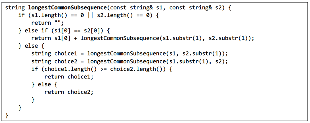
longestCommonSubsequence
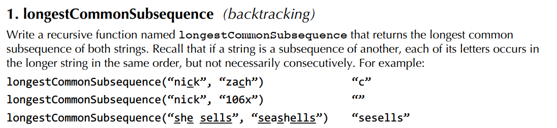
这道题类似于Assignment 4的最后一个问题,是一个subSet问题。这种问题的一般想法是:对于某个位置的某个元素,include or not? 之后再针对include/not include的两种情况的大小或者其他条件,将各自作为返回值:
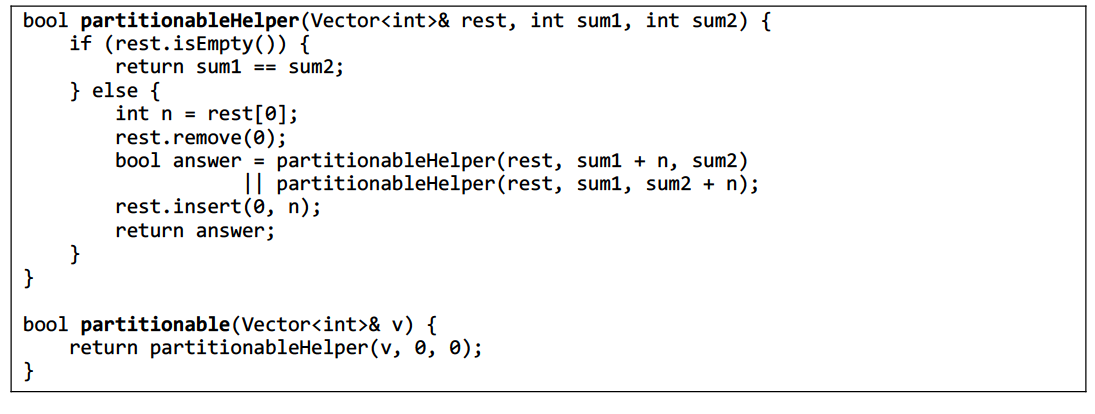
partitionable
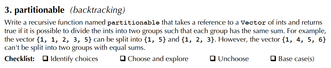
这道题的解法不止一种,最初我的方法是将这道题转化为dicsSum来做,而答案则是转化成了一个类似于include or not的方法来做:对于每一个元素,我们可以选择加入sum1或者选择加入sum2,答案的写法是比较精妙的:
这道题的处理让我想起在CS 61A中期末复习题中的一道题目(lab14 q4):
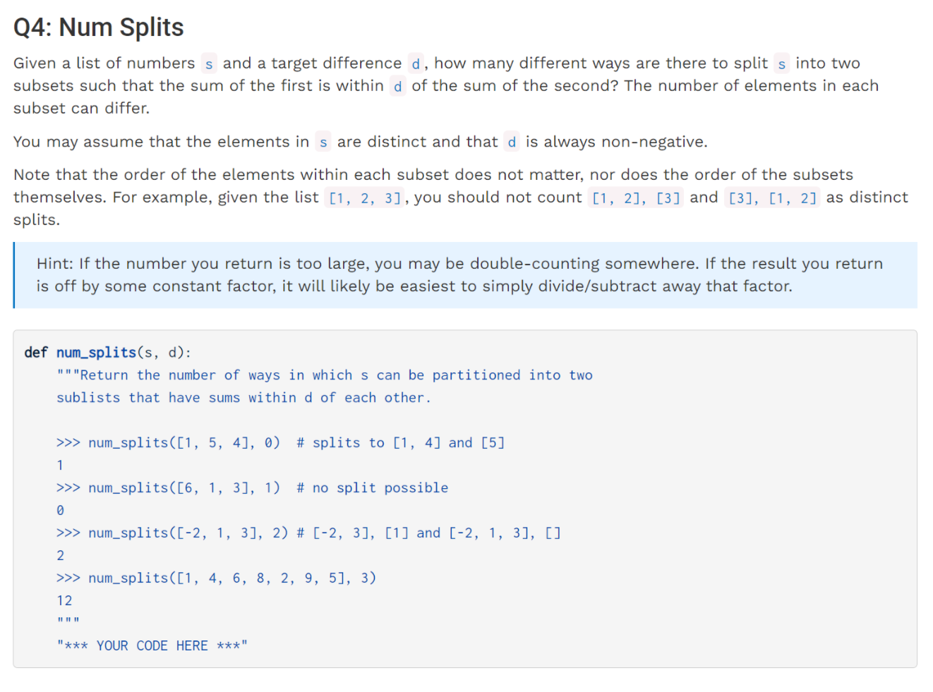
这道题也可以使用这种方法来做:
int subSeq(const vector<int>& test, int d) {
    vector<int> test1 = test;
    return subSeqHelepr(test1, 0, 0, d);
}

int subSeqHelepr(vector<int>& test, int sum1, int sum2, int d) {
    if (test.empty()) {
        return abs(sum1 - sum2) <= d;
    }
    else {
        int first = test[0];
        test.erase(test.begin());
        int result = subSeqHelepr(test, sum1 + first, sum2, d) + subSeqHelepr(test, sum1, sum2 + first, d);
        test.insert(test.begin(), first);
        return result;
    }
}
listTwiddles
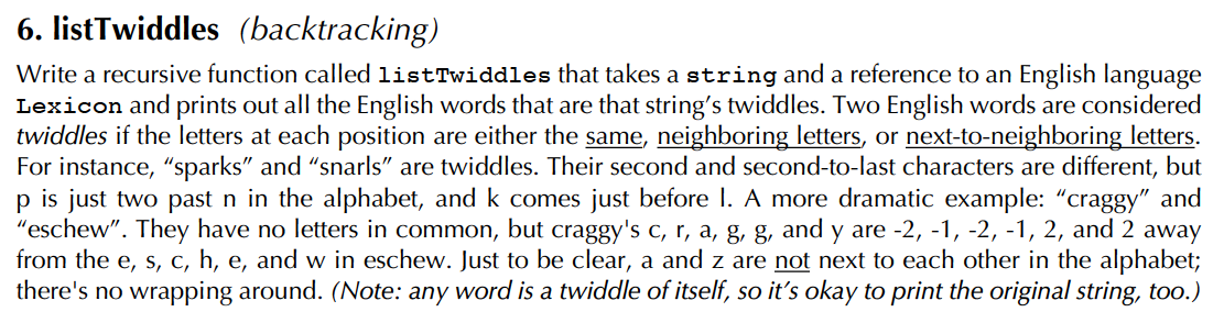
我们经常会遇到一些数据量比较大的递归问题,此时我们的选择不应当是在函数中直接遍历,比如此题中的lexicon,也比如在Assignment 4的第二个问题,我们应当遍历的都是针对题目所谓的neighbors。在Assignment 4中,对大数据集unCovered的处理是通过改变函数参数,将此次函数使用的neighbors去除实现的;而在本题中,则增加了一个参数index来实现对Lexicon的持续遍历。
Section 4 & 5 - linked list
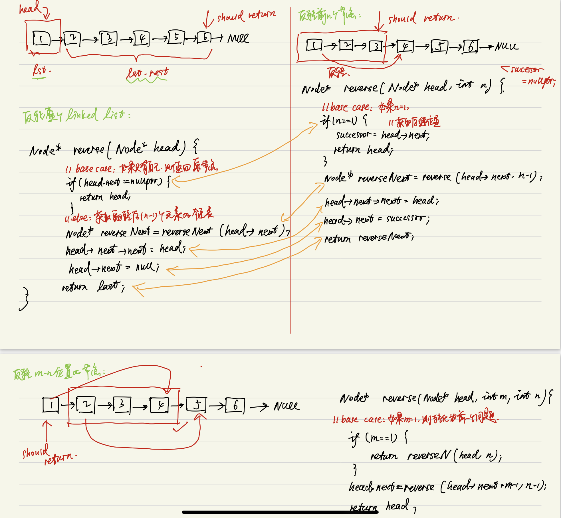
reverse linked list
首先通过一个例子来展示链表反转的过程:

为了实现链表反转,我们需要从末尾入手,这其实也比较像是递归的思路,先遍历到最后,再回溯到链表的头部,所以我们也可以使用递归代码来解决这个问题。
在此例中,如果我们想翻转这三个节点,需要做如下操作:
// set the pointer at the end of the list
listNode* temp = list->next->next;
// connect one node to the new temp node
temp->next = list->next;
// 4->5
list->next->next = list;
// set the end of null
list->next->next->next = nullptr;
list = temp;
通过上图所示这种,自后往前的反转方法,我们可以将问题扩展到如下三个层次:并分别作了如下解析:
// 一个反转链表的函数变体
void reverse(listNode*& front) {
    if (front == nullptr || front->next == nullptr) {
        return;
    }
    listNode* temp = front->next;
    // 因为是传递引用,所以最终temp的值会等于最后一个element
    reverse(temp);
    front->next->next = front;
    front->next = nullptr;
    // 设置新的链表头部位置
    front = temp;
}
remove elements
之所以把这一条单独列出来,是因为在删除元素的过程中,我们常需要将删除链表的头部元素这一操作从删除过程中独立出来。同时,在删除元素时,我们也要注意不要遍历到链表的nullptr位置,否则无法将链表前后相互连接起来:
void removeAllThreshold(ListNode*& front, int value, int threshold) {
    // deal with the front delete case
    while (front != nullptr && front->data >= value - threshold
          				   && front->data <= value + threshold) {
        listNode* trash = front;
        front = front->next;
        delete trash;
    }
    // normal delete case
    if (front != nullptr) {
        listNode* current = front;
        while (list->next != nullptr) {
            if (current->next->data >= value - threshold
                && current->next->data <= value + threshold) {
                listNode* trash = current->next;
                current->next = current->next->next;
                delete trash;
            }
            else {
                current = current->next;
            }
        }
    }
}
split
将链表中的数据分组,比如分为正数和负数,且在操作过程中不创建任何新节点,这意味着我们需要对连接链表前后数据的指针进行不断的调整和移动:所以我们的思路是,当遇到一个负数时,就把该节点的下一个节点设置在当前的front位置,在操作结束后,就把front设置到当前节点的位置,如此一来,负数节点便可以连接在一起,紧随其后的是非负数节点:
void split(ListNode*& front) {
    if (front != nullptr) {
        listNode* current = front;
        while (current->next != nullptr) {
            if (current->next->data < 0) {
                listNode* temp = current->next;
                current->next = current->next->next;
                temp->next = front;
                front = temp;
            }
            else {
                current = current->next;
            }
        }
    }
}
braid
简而言之,就是要将先前的链表与翻转之后的链表交叉连接在一起:
此类题目,我们常需要用到stack、queue等数据结构。而在本题中,可以预想到的思路是先遍历到原链表末尾,之后把头部元素加入,这就需要FIFO的功能,所以应当使用队列而非堆栈。
我们可以通过思考在链表末尾添加元素的simple case来验证正确性
void braid(listNode* front) {
    Queue<int> numbers;
    braidHelper(front, numbers);
}

void braidHelper(listNode* front, Queue<int>& numbers) {
    // base case
    if (front == nullptr) {
        return;
    }
    numbers.enqueue(front->data);
    // use recursion to store all nodes' data in the queue
    braidHelper(front->next, numbers);
    // insert the node's data into the right position in the current linked list
    listNode* newNode = new listNode(numbers.dequeue(), front->next);
    // connect the list
    front->next = newNode;
}
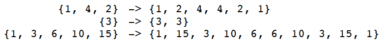
奇偶链表
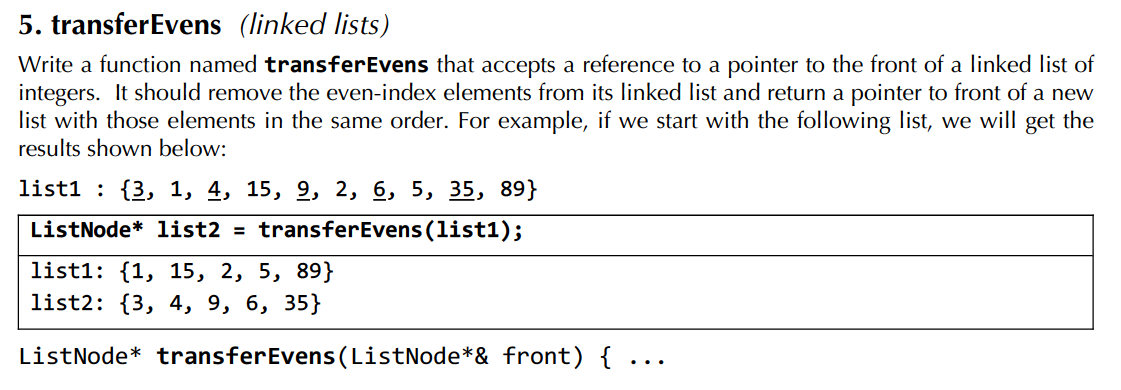
可以想到,除了原指针list1之外,我们至少还需要两个指针分别用于对偶数位节点的跟随与之后的遍历;同样地,为了跟随奇数位节点,我们需要再创立一个新节点(这个题最好的解法就是把图画出来,对照着写码):
ListNode* transferEvens(ListNode*& list1) {
    if (list1 == nullptr) {
        return nullptr;
    }
    // the head for even sequence
    ListNode* list2 = list1;
    // the head for odd sequence
    list1 = list1->next;
    // keep track of the even sequence
    ListNode* even = list2;
    // keep track of the odd sequence
    ListNode* odd = list1;
    // start traversing:
    while (odd != nullptr && odd->next !+ nullptr) {
        even->next = odd->next;
        even = even->next;
        odd->next = even->next;
        odd = odd->next;
    }
    even->next = nullptr;
    return list2;
}
Section 6 - Binary Search Tree
IsBST
这个类型的题目在Berkeley CS 61A中见到过,这里给出完整的判定方法:
bool isBST(TreeNode* node, int min, int max) {
    if (node == nullptr) {
        return true;
    }
    if (node->data <= min && node->data >= max) {
        return false;
    }
    return isBST(node->left, min, node->data) && isBST(node->right, node->data, max);
}
WordExists
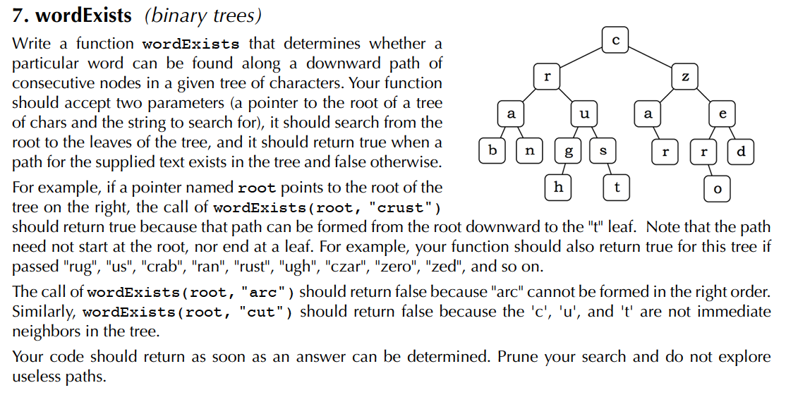
这道题我的思路是将其理解为一个回溯问题,因为它并不要求单词的起始节点位于根节点处,所以当我们在某一分支中没有完全匹配该单词时,我们需要到另一分支中寻找原单词。基于这种考虑,设置一个辅助参数,保留未经更改的原单词:
bool wordExists(TreeNodeChar* node, const string& word) {
    return wordExistsHelper(node, word, word);
}
bool wordExistsHelper(TreeNodeChar* node, string originalWord, string word) {
    if (word.empty()) return true;
    if (node == nullptr) return false;
    // is now we found a match char
    if (node->data == word[0]) {
        // choose
        return wordExistsHelper(node->left, originalWord, word.substr(1)) ||
                wordExistsHelper(node->right, originalWord, word.substr(1));
    }
    else {
        // un-choose
        return wordExistsHelper(node->left, originalWord, originalWord) ||
                wordExistsHelper(node->right, originalWord, originalWord);
    }
}
当然,我们也可以选择不保留原本的单词,那么我们需要将在某一分支中判定是否存在完美匹配的单词这一过程独立出来,否则会出现误判的情况:
// helper to search the given subtree for the rest of the string bool
suffixExists(TreeNodeChar* node, const string& suffix) {
   if (suffix.empty()) {
        return true;
    }
    else if (node == nullptr) {
        return false;
    }
    else if (suffix[0] != node->data) {
        return false;
    }
    else {
        return suffixExists(node->left,  suffix.substr(1)) ||
            suffixExists(node->right, suffix.substr(1));
    }
}
bool wordExists(TreeNodeChar* node, const string& str) {
    if (str.empty()) {
        return true;
        // the empty tree contains the empty string
    }
    else if (node == nullptr) {
        return false;
    }
    else if (suffixExists(node, str)) {
        return true;
    }
    else { return wordExists(node->left, str) ||
        wordExists(node->right, str); }
}
二叉搜索树转双向链表
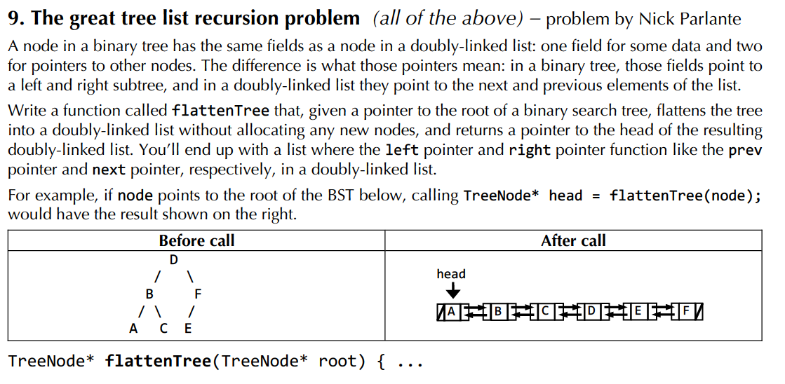
这是一道十分经典的数据结构题目,《剑指offer》上对此题有详细描述,利用了二叉树中序遍历不改变节点大小顺序的性质。这里只贴代码:
TreeNode* flattenTree(TreeNode* root) {
    TreeNode* lastNodeInList = nullptr;
    // since we perform in-order traversal, so we will return the last node in the list
    convertNode(root, lastNodeInList);
    // we need to return the head
    TreeNode* head = lastNodeInList;
    while (head != nullptr && head->left != nullptr) {
        head = head->left;
    }
    return head;
}

void convertNode(TreeNode* root, TreeNode*& node) {
    if (root == nullptr) {
        return;
    }
    // left
    if (root->left != nullptr) {
        convertNode(root->left, node);
    }
    // link the root into the current link list
    root->left = node;
    if (node->right != nullptr) {
        node->right = root;
    }
    // set the root as the current lastNode
    node = root;
    // right
    if (root->right != nullptr) {
        convertNode(root->right, node);
    }
}
刚开始有些疑惑,为什么这里有把左子树连接到根节点但是却没有将右子树连接到根节点的过程?这也是使用中序遍历的便利之处,我们所有的操作在两次遍历之间完成。其实如果要去分析也很容易,因为链接的信息是被我们保存在了
node数据中,在右子树的遍历过程中,会利用该参数的信息,将右子树的最小节点与根节点(即node)链接起来。
Section 7 - Graph
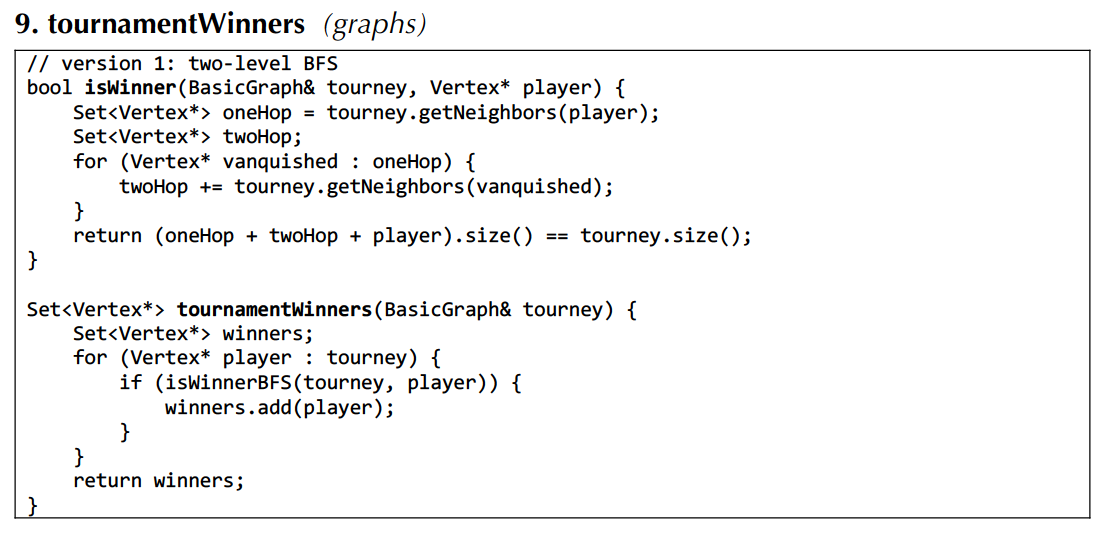
tournamentWinners

这道题对winner的判定方法比较巧妙,通过比较size实现:
DFS + memorization (岛屿问题?)
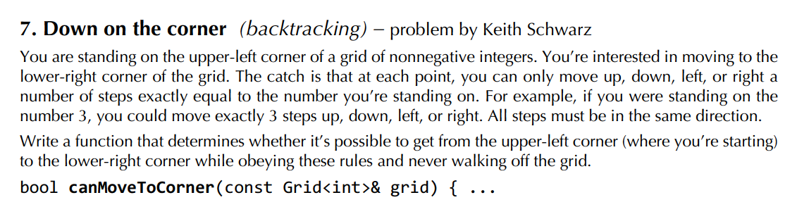
这道题目的关键在于单独设置一个二维的visited数组,用于表示之前是否到达过该点,如果到达过,那么直接返回(因为使用DFS,相当于所有从该点继续往后走的情况都被探查过了):
// use Stanford C++ library
bool canMoveToCornerHelper(const Grid<int>& grid, int i, int j, Grid<bool>& visited) {
    if (!grid.inBounds(i, j)) {
        return false;
    }
    if (visited[i][j]) {
        return false;
    }
    // if get to the place, return
    if (i == (grid.numRows() - 1) &&
            j == (grid.numCols() - 1)) {
        return true;
    }
    // recursion
    // get the number:
    int step = grid[i][j];
    visited[i][j] = true;
    // four choices, perform backtracking
    if (canMoveToCornerHelper(grid, i - step, j, visited)
            || canMoveToCornerHelper(grid, i + step, j, visited)
            ||  canMoveToCornerHelper(grid, i, j - step, visited)
            || canMoveToCornerHelper(grid, i, j + step, visited)) {
        return true;
    }
    return false;
}

bool canMoveToCorner(const Grid<int>& grid) {
    // keep track of the path
    Grid<bool> visited(grid.numRows(), grid.numCols());
    visited.fill(false);
    return canMoveToCornerHelper(grid, 0, 0, visited);
}
BFS的灵活运用
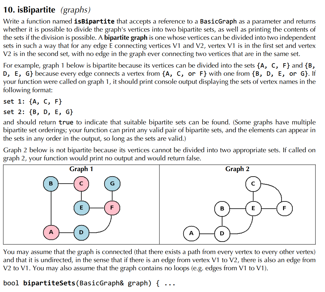
这道题思路向BFS靠拢,但是要对BFS做一点改变,同时注意这里我们需要的是遍历,而不是去求最短路径,所以不需要设置终止条件:
bool isBipartite(const BasicGraph& graph) {
    Set<Vertex*> vertexSet = graph.getVertexSet();
    // store two bipartite sets
    Set<string> red, blue;
    // track which set vertices are in, if any
    Map<Vertex*, string> colorMap;
    // queue in BFS
    Queue<Vertex*> queue;
    // perform BFS
    Vertex* first = vertexSet.first();
    colorMap[first] = "r";
    queue.enqueue(first);
    red.add(first->name);
    while (!queue.isEmpty()) {
        Vertex* node = queue.dequeue();
        Set<Vertex*> neighbors = graph.getNeighbors(node);
        for (auto& neighbor : neighbors) {
            // if un-visited
            if (!colorMap.containsKey(neighbor)) {
                // set the opposite color to the node's
                if (colorMap[node] == "r") {
                    colorMap[neighbor] = "b";
                    blue.add(neighbor);
                }
                else {
                    colorMap[neighbor] = "r";
                    red.add(neighbor);
                }
                queue.enqueue(neighbor);
            }
            // if visited, check its color
            else if (colorMap[node] == colorMap[neighbor]) {
                return false;
            }
        }
    }
    // cout sth.

    return true;
}
CS 106X Lecture 16-18 & UIUC CS 225 – Trees
在这里对一些可能面试会用到的树的类型做一个总结:
对于一棵二叉树来讲,我们可以通过DFS和BFS两种方法对树进行搜索(或者进行遍历)。考虑search这一操作:我们可以得到如下的时间复杂度与空间复杂度(均指最坏情况):
| 时间复杂度 | 空间复杂度 | |
|---|---|---|
| DFS | O(n) | O(h) |
| BFS | O(n) | O(n) |
在讨论时,主要考查完美二叉树以及h=n的特殊情况,对于空间复杂度的分析通过计算实现DFS与BFS操作的栈内节点数量得到。如果我们使用递归实现,那么求的是递归最深的那一次压栈所耗费的空间的个数;递归最深的那一次所耗费的空间足以容纳它所有递归过程。
Binary Search Tree (BST)
基本数据结构
class BST {
    public:
    // remove
    // insert
    // getMin
    //...

    private:
    // a node data structure
        struct TreeNode {
            int value;
            TreeNode* left, right;
            // a constructor
            TreeNode(int value, TreeNode* left = nullptr, TreeNode* right = nullptr)
            {};
        };
        // head pointer
        TreeNode* head;
};
二叉搜索树具备以下特征:
- left.v < p.v < right.v
- O(lgn) < O(V) < O(h)
方法实现
contains-O(h)
bool contains(TreeNode*& node, int value) {
    if (node != nullptr) {
        if (node->data == value) {
            return true;
        }
        bool result = contains(node->left, value) ||
            contains(node->right, value);
        if (result) {
            return true;
        }
    }
    return false;
}
search-O(h)
TreeNode* find(TreeNode*&, int value) {
    if (node != nullptr) {
        if (value < node->data) {
            return find(node->left, value);
        }
        else if (value > node->data) {
            return find(node->right, value);
        }
        else {
            return node;
        }
    }
    return nullptr;
}
getMin-O(h)
最小值存在于树的最左侧节点,同理,最大值为树的最右侧节点
// pass by pointer(value)
int getMin(TreeNode* node) {
    if (node->left != nullptr) {
        return getMin(node->left);
    }
    else
        return node->data;
}
insert-O(h)
void insert(TreeNode*& node, int value) {
    if (node != nullptr) {
        if (value > node->data) {
            insert(node->right, value);
        }
        else if (value < node->data) {
            insert(node->left, value);
        }
        else {
            // do nothing, don't need to insert
            return;
        }
    }
    node = new TreeNode(value);
}
remove-O(h)
当所删除节点有两个孩子时,主要流程包括:
- 先找到删除节点
- 找到该节点的前驱(左子树中的最大节点)或者后继(右子树中的最小节点)
- swap
- 删除交换后的原节点
void remove(TreeNode*& node, int value) {
    if (node == nullptr) return;
    if (value > node->data) {
        remove(node->right, value);
    }
    else if (value < node->data) {
        remove(node->left, value);
    }
    // different removing cases
    else {
        // case 1: leaf
        if (node->isLeaf()) {
            // free the memory that the current node pointing at
            delete node;
            // set the node pointing to null, indicating node's parent
            // that there is no child
            node = nullptr;
        }
        // case 2: only left subtree
        else if (node->right == nullptr) {
            TreeNode* trash = node;
            node = node->left;
            delete trash;
        }
        // case 3 : only right subtree
        else if (node->left == nullptr) {
            TreeNode* trash = node;
            node = node->right;
            delete trash;
        }
        // case 4: have two children
        else {
            // find IOS
            int minValue = getMin(node->right);
            node->data = minValue;
            remove(node->right, minValue);
        }
    }
}
AVL Tree (Balanced Tree)
基本特征
Height balance:
b = height(Tr) - height(Tl)
A tree is balanced if: The tree itself and all its subtrees meets:
$$\lvert b \rvert \le 1$$.
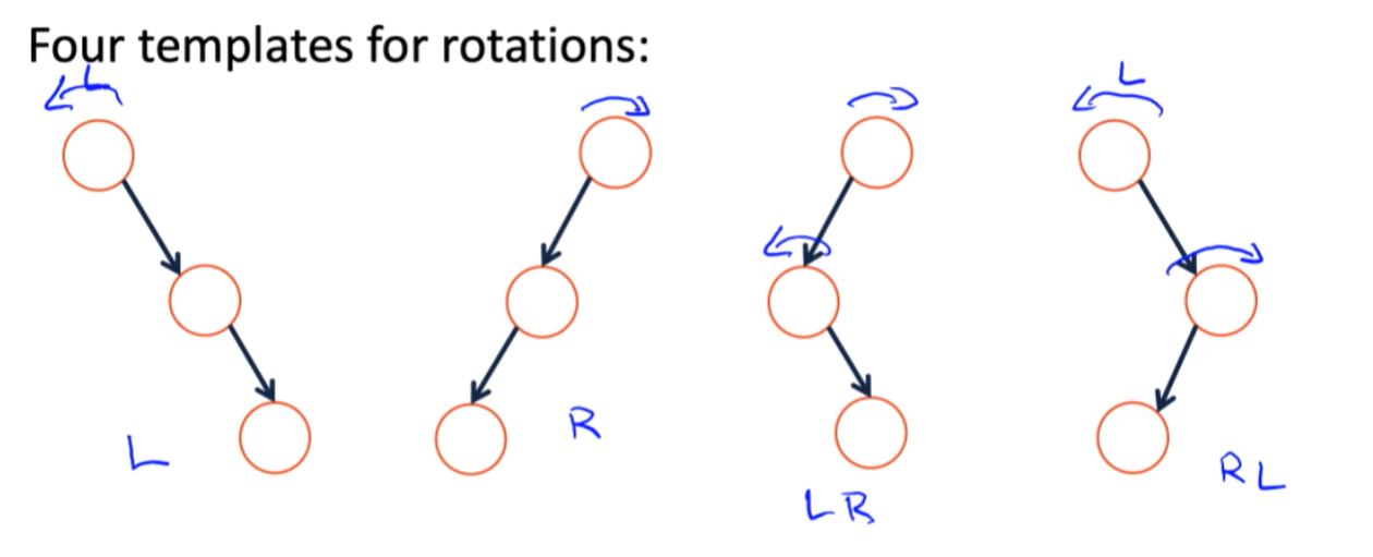
- Four kinds of rotations (L, R, LR, RL)
- All rotations are local (subtrees are not impacted)
- All rotations are constant time: O(1)
- BST property maintained
rotation example
- L
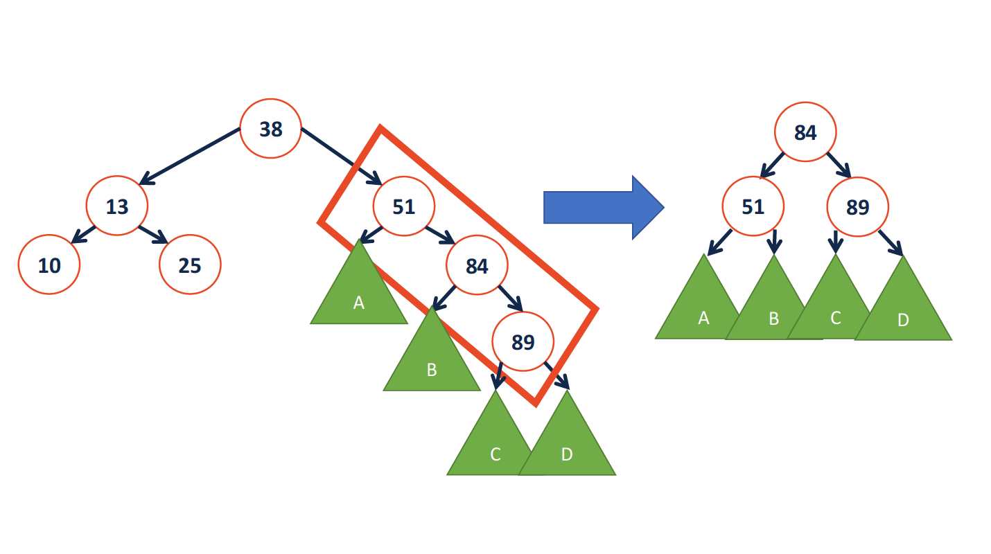
只需要更改3处指针,所以旋转的操作时间复杂度为常数级
- LR
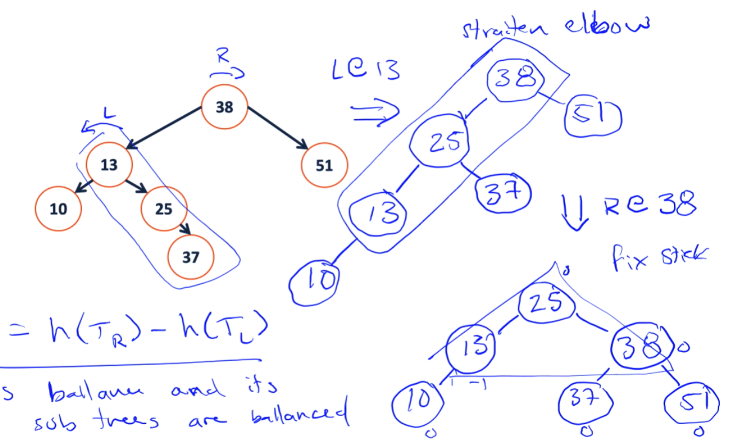
需要注意的几个变换特征:
- 对于单独的左旋转与右旋转,我们所处理的对象是一个stick;而对于两种复合操作来说,我们所处理的对象形状被定义为一个elbow。
- 分别观察左旋转与右旋转,我们容易发现,它们都是以stick的中心节点为轴,左旋转将stick中的顶端节点转到左下端,而右旋转则成对称式地将位于右上的顶端节点旋转到右下方。他们最后都形成一个山峰状。
- 对于此类复合型操作,在图像上的效果也是先展开再弯曲.从操作上来讲,是先对中间节点进行左旋(右旋),之后再对整体(子树根节点)进行右旋(左旋)。
finding rotations on Insert
- L
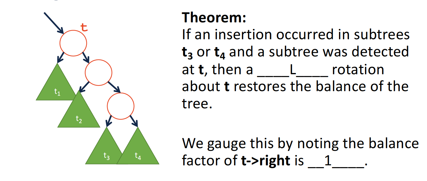
因为在插入节点后,平衡标志的计算是自顶而上的,在第一次检测到不满足AVL条件的位置t,平衡系数b一定为2.
继续推断得到:t->right的b值为1.
- RL
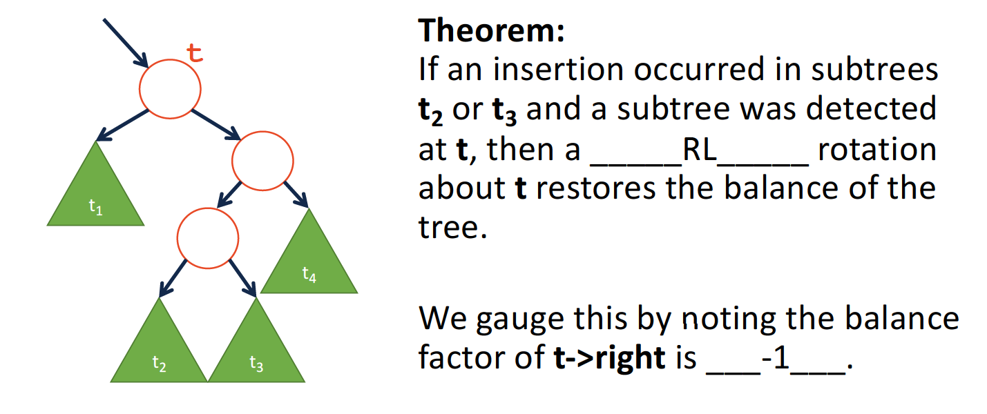
同理,对于这一类旋转,t位置b为2,但是t->right的b为**-1**.
基本数据结构
struct TreeNode {
    int data;
    // need to keep track of the node's height
    unsigned height;
    TreeNode* left;
    TreeNode* right;
}
方法实现
height-O(1)
int height(TreeNode* node) {
    if (node == nullptr) {
        return 0;
    }
    return node->height;
}
rightRotate-O(1)
void rightRotate(TreeNode*& node) {
    TreeNode* x = node->left;
    TreeNode* t2 = x->right;

    // perform rotation
    x->right = node;
    node->left = t2;

    // update the heights
    node->height = max(height(node->left), height(node->right)) + 1;
    x->height = max(height(x->left), height(x->right)) + 1;
}
leftRotate-O(1)
void leftRotate(TreeNode*& node) {
    TreeNode* x = node->right;
    TreeNode* t2 = x->left;

    // preform rotation
    x->left = node;
    node->right = t2;

    // update the height
    node->height = max(height(node->left), height(node->right)) + 1;
    x->height = max(height(x->left), height(x->right)) + 1;
}
reBalance-O(lgn)
void rebalance(TreeNode*& node) {
    // calculate two balances
    int balance = height(t->right) - height(t->left);

    if (balance == 2) {
        int rightBalance = height(node->right->right) - height(node->right->left);
        if (rightBalance == 1) {
            // R
            leftRotate(node);
        }
        else if (rightBalance == -1) {
            // RL
            rightRotate(node->right);
            leftRotate(node);
        }
    }
    else if (balance == -2) {
        int leftBalance = height(node->left->right) - height(node->left->left);
        if (leftBalance == -1) {
            // R
            rightRotate(node);
        }
        else if (leftBalance == 1) {
            // LR
            leftRotate(node->left);
            rightRotate(node);
        }
    }
    // update the t's height
    node->height = max(height(node->left), height(node->right)) + 1;
}
insert-O(lgn)
AVL树的插入操作可以被分为四个步骤:
- Insert at proper place
- Check for imbalance
- Rotate, if necessary
- Update height
- Recursive up
void insert(TreeNode*& node, int value) {
    // insert
    if (node == nullptr) {
        node = new TreeNode(value);
    }
    // will insert and adjust the right tree
    else if (value > node->data) {
        insert(node->right, value);
    }
    // will insert and adjust the left tree
    else if (value < node->data) {
        insert(node->left, value);
    }
    // rebalance the tree
    reBalance(node);
}
为什么插入操作只需要对树进行一次reBalance,因为插入会将树的高度增加1,而重平衡会将树的高度减短1,故不会对其余部分造成影响。
remove-O(lgn)
void remove(TreeNode*& node, int value) {
    // use the BST remove function
    remove(node, value);
    // reBalance the tree (each subtree)
    reBalance(node);
}
复杂度分析
这一部分可以参见UIUC CS 225关于AVL树的性能分析,通过节点数目与树的高度的关系得到了一个粗略的下界,反过来确定了树高度的上界(一个估计值)。这里不作详细讨论。
Tries (Dictionary Search Tree)
基本数据结构
struct TireNode {
    TrieNode* chilren[26];
    bool isWord;
}
单词查找树的特点在于:查找命中所需的时间与被查找的键的长度成正比。(如果我们将字母存储于一个二叉平衡搜索树中,则查找需要的时间为键的长度*O(lgn))
方法实现(My Github)
由于字典查找树的实现较为复杂,我将实现方法放到了我的GitHub仓库中,该仓库内同时包含了压缩字典查找树,即compressed trie的实现。
关于compressed trie,这里有一篇博客讲得比较清楚,我的代码也是根据此原理实现:
http://theoryofprogramming.com/2016/11/15/compressed-trie-tree/
KD-Tree & BTree
这部分内容不作详细实现了,KD-Tree准备在CS 106L课程中实现,B树的性质讲解可以参见UIUC CS 225的课程视频。这里仅仅列出关于B树的一部分内容:
B树性质
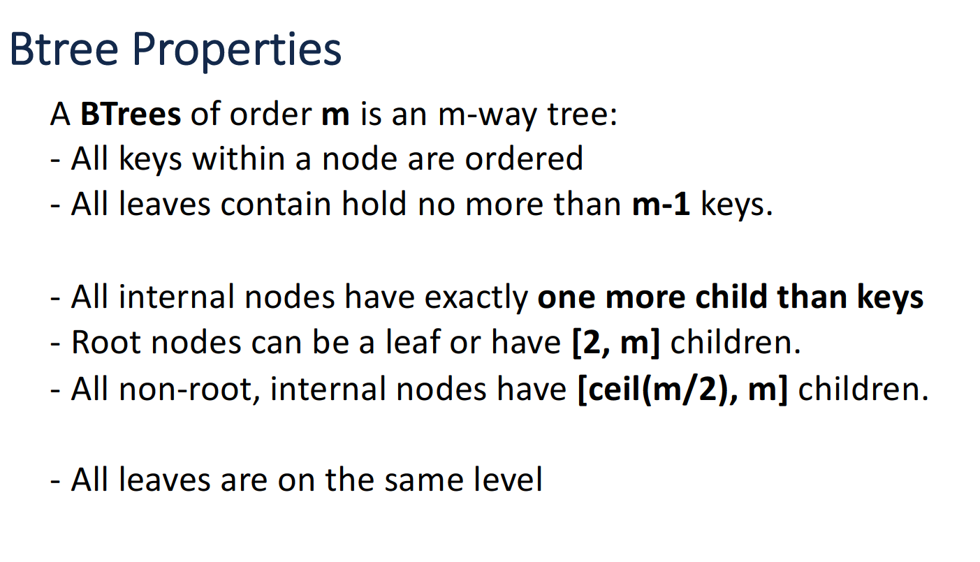
insert & search
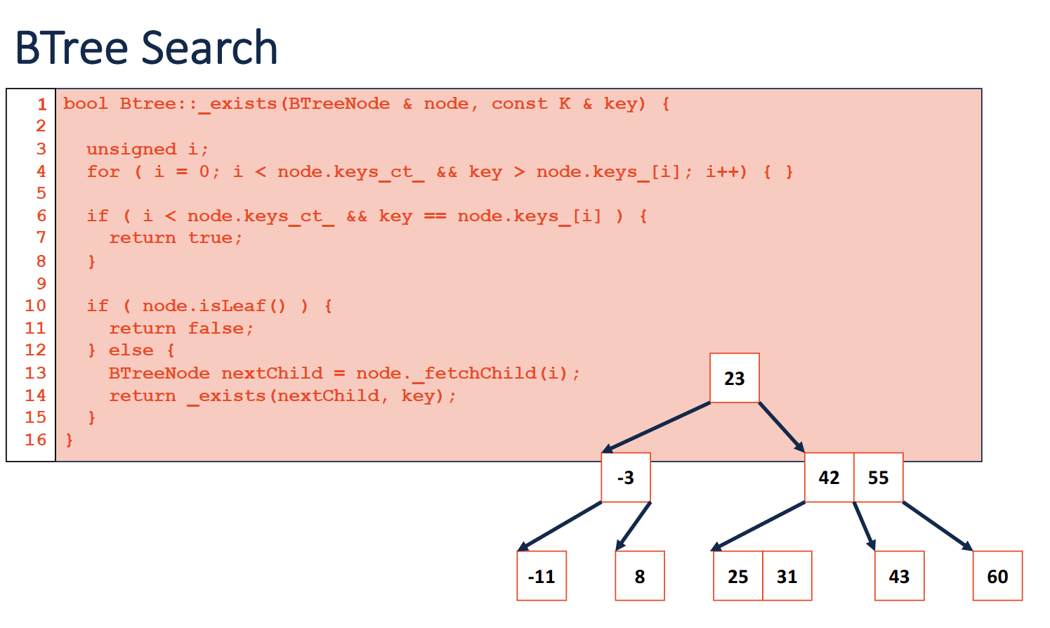
这段代码的思路其实也很好理解,先找到所查看节点中的合理位置,之后再根据情况进行递归即可,或者直接返回结果。
而B树的插入是一个自底向上的过程,首先找到该层节点中合适的位置,之后我们通过递归不断变更节点的祖先(如果有必要)。
Segment Tree
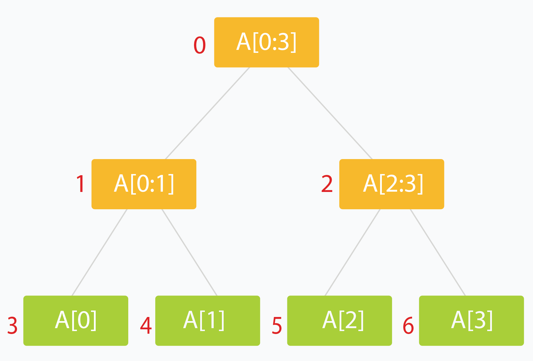
线段树常被用于存储区间,使用该结构来对区间进行操作,比如查询或者更新。线段树的常见构造有:父节点为两子节点的最小值、最大值或者他们的和。这里以min query为例,进行探讨。
construct-O(n)
关于线段树的构造,网上教程很多,这里仅列出几点,为了避免日后自己忘记:
- 线段树的构造与堆类似,并不是用真正的树结构存储,而是是用了数组的方法,并通过下标的换算来决定父节点和子代节点的位置。两个子节点的坐标分别为:$$2i+1$$和$$2i+2$$.
- 如果给定目标数组的维度为$$n$$,那么我们需要找到线段树的维度$$N$$,满足$$N=2*k-1$$,其中$$k$$满足$$min(k-n)$$,且$$k=2^q$$。
- 由于我们处理的节点数(根据前边的公式)大致为$$2n$$个,所以构造过程的时间复杂度为O(n)。
- 仍然是通过递归的方法构造,这也得益于线段树的父节点与子节点的关系特性。
- 构造过程也是自底向上的。
SegmentTree::SegmentTree(const int * array, int n) {
    // get the next power of 2
    int powerSize = nextPowerOf2(n);
    // allocate the memory to the private member array
    // based on the attribute of segmentTree
    segmentTree = new int[powerSize * 2 - 1];
    // store the INT_MAX
    for (int i = 0; i < powerSize; ++i) {
        segmentTree[i] = INT_MAX;
        // also initialize the lazy array
        lazy[i] = 0;
    }
    constructHelper(array, 0, n - 1, 0);
}
void SegmentTree::constructHelper(const int * array, int low, int high, int pos) {
    // we reach the end of the segmentTree
    if (low == high) {
        segmentTree[pos] = array[low];
        return;
    }
    int mid = (low + high) / 2;
    int leftChildPos = 2 * pos + 1;
    int rightChildPos = 2 * pos + 2;
    constructHelper(array, low, mid, leftChildPos);
    constructHelper(array, mid + 1, high, rightChildPos);
    // after the left & right children are all being processed, set the parent
    segmentTree[pos] = min(segmentTree[leftChildPos], segmentTree[rightChildPos]);
}
nextPowerOf2
该辅助函数使用位操作帮助找到距离
$$n$$最近的2的次幂。
unsigned int nextPowerOf2(int n) {
    unsigned int result = 1;
    // n is a power of 2
    // using bits operation
    if (n && !(n & (n - 1))) {
        return n;
    }
    // else
    while (result < n) {
        result <<= 1;
    }
    return result;
}
rangeMinQuery-O(lgn)
该函数的功能是进行区间查找,找到区间的最小值。对于此类问题,有以下几个注意点:
- 此类问题以及后边即将出现的区间更新,其时间复杂度均为对数级别
- 此类问题以及后边即将出现的区间更新,均被分为三种情况予以讨论:no overlap, total overlap, partial overlap,分别对应了代码中的base case以及recursive case。**但要注意的是,这里的重合情况的对象是由给定区间指向总长度的,而非查看总长度相对于给定区间的重合情况。**在部分重合时,我们需要继续递归,其目的也就是为了找到total overlap的位置。
int SegmentTree::rangeMinimumQueryHelper(const int *array, int low, int high, int qlow, int qhigh, int pos) {
    // no overlap
    if (qlow > high || qhigh < low) {
        return INT_MAX;
    }
    // total overlap
    if (qlow >= low && qhigh <= high) {
        return segmentTree[pos];
    }
    // partial overlap
    // continue to search
    int mid = (low + high) / 2;
    int leftChildPos = 2 * pos + 1;
    int rightChildPos = 2 * pos + 2;
    // since it is min query
    return min(rangeMinimumQueryHelper(array, low, mid, qlow, qhigh, leftChildPos),
               rangeMinimumQueryHelper(array, mid + 1, high, qlow, qhigh, rightChildPos));
updateTreeRange-O(lgn)
效仿上边的方法,有所不同的是,当遇到no overlap的情况时,我们应当直接返回,而不是提供一个MAX标记。
void SegmentTree::updateSegmentTreeRangeHelper(int low, int high, int qlow, int qhigh, int pos, int delta) {
    // put the low>high(an error case in final) case and the "no overlap" case together
    if (low > high || qlow > high || qhigh < low) {
        return;
    }
    // reach the end
    if (low == high) {
        segmentTree[pos] += delta;
    }
    int mid = (low + high) / 2;
    int leftChildPos = 2 * pos + 1;
    int rightChildPos = 2 * pos + 2;
    updateSegmentTreeRangeHelper(low, mid, qlow, qhigh, leftChildPos, delta);
    updateSegmentTreeRangeHelper(mid + 1, high, qlow, qhigh, rightChildPos, delta);
    segmentTree[pos] = min(segmentTree[leftChildPos], segmentTree[rightChildPos]);
}
lazy propagation
lazy propagation是线段树中的一种重要的优化操作,通俗一点说,lazy propagation可以让我们再区间更新时,不需要在树的某一分支中从顶到下的更新所有区内节点,我们可以只更新到total overlap的位置(之后便可以返回了,这也是符合直观感受和线段树的节点意义的),并在lazy tree中的子代节点处设置一个对应的本次更新值, 意味着以下的数据不是最新的。当以后有必要查询和更新时,再逐步将先前的更新值传递到下层的节点当中。
updateTreeRangeLazy
void SegmentTree::updateSegmentTreeRangeLazyHelper(int low, int high, int qlow, int qhigh, int pos, int delta) {
    // an error case, we cannot combine this case with the no overlap case
    // when doing lazy propagation, since we need to check the lazy tree first
    // even when no overlap
    if (low > high) {
        return;
    }
    if (lazy[pos] != 0) {
        // send the past operation's result back to the segmentTree node
        segmentTree[pos] += lazy[pos];
        // we are not at the position of leaf node
        if (low != high) {
            lazy[2 * pos + 1] += lazy[pos];
            lazy[2 * pos + 2] += lazy[pos];
        }
        // eliminate the past flag at pos
        lazy[pos] = 0;
    }
    // no overlap
    if (qlow > high || qhigh < low) {
        return;
    }
    // total overlap
    if (qlow >= low && qhigh <= high) {
        segmentTree[pos] += delta;
        // doing lazy propagation
        if (low != high) {
            lazy[2 * pos + 1] += delta;
            lazy[2 * pos + 2] += delta;
        }
        // immediately return
        return;
    }
    // partial overlap
    int mid = (low + high) / 2;
    int leftChildPos = 2 * pos + 1;
    int rightChildPos = 2 * pos + 2;
    updateSegmentTreeRangeLazyHelper(low, mid, qlow, qhigh, leftChildPos, delta);
    updateSegmentTreeRangeLazyHelper(mid + 1, high, qlow, qhigh, rightChildPos, delta);
    segmentTree[pos] = min(segmentTree[leftChildPos], segmentTree[rightChildPos]);

}
而当我们进行查询时,就也需要对应的操作了:
int SegmentTree::rangeMinimumQueryLazyHelper(const int *array, int low, int high, int qlow, int qhigh, int pos) {
    // an error case might encounter at leaf node
    if (low > high) {
        return INT_MAX;
    }
    // see the lazy tree, if there is some states we have not performed in our
    // segment tree ever?
    if (lazy[pos] != 0) {
        // need to pass back the update result from the lazy tree to the segment tree
        segmentTree[pos] += lazy[pos];
        if (low != high) {
            // update the lazy tree state to the next level
            lazy[2 * pos + 1] += lazy[pos];
            lazy[2 * pos + 2] += lazy[pos];
        }
        lazy[pos] = 0;
    }
    // no overlap
    if (qlow > high || qhigh < low) {
        return INT_MAX;
    }
    // total overlap
    if (qlow >= low && qhigh <= high) {
        return segmentTree[pos];
    }
    // partial overlap
    // continue to search
    int mid = (low + high) / 2;
    int leftChildPos = 2 * pos + 1;
    int rightChildPos = 2 * pos + 2;
    // since it is min query
    return min(rangeMinimumQueryLazyHelper(array, low, mid, qlow, qhigh, leftChildPos),
               rangeMinimumQueryLazyHelper(array, mid + 1, high, qlow, qhigh, rightChildPos));
}
Heap
本部分内容参照《算法导论》
private:
    // TODO: add specified member variable(s)
    // current size
    int size;
    // total size of the heap
    int capacity;
    // the heap pointer
    PatientNode* heap;
二叉堆是一个数组,可以被近似为一个完全二叉树。除了最底层之外,该树是完全充满的。为了方便数学运算,我们从index=1开始存储堆元素,在segment tree那里我们也提到过这种存储方式,但是两者的存储方法稍有不同,导致在堆中i节点的父节点位置为[i/2],左右子节点分别为:2i, 2i+1.
堆的一个特性是:含有n个元素的堆的高度为[lgn]
这一特性的证明可以通过利用完全二叉树的性质,利用夹逼定理进行证明,即不等式:
$$2^{h+1} - 1> n > 2^h$$
**最小堆是构造优先队列的常用方法。**在CS 106X的课程作业中,也出现了这一主题,分别使用链表与堆构建优先级队列. 这里就以构建最小堆为例,讨论堆的各种操作与实现方法:
在以下的实现方法中,函数参数包含了指向
heap的指针,是为了方便独立参照。
MIN-HEAPIFY-O(lgn)
这一操作是维护堆性质的重要过程,输入为一个数组A和一个下标i,因为父节点有可能大于它的子节点,所以要在堆中“逐级下降”(downheap):
主要过程是先找到当前节点以及其两个子结点中最小的,如果最小的节点不是当前节点,而是两个子结点中的一个,那么我们需要交换他们,并进一步的,对子堆递归下去。
void minHeapify(int size, int i) {
    int smallest = i;
    int left = 2 * i;
    int right = 2 * i + 1;
    if (left <= size && heap[smallest] > heap[left]) {
        smallest = left;
    }
    if (right <= size && heap[smallest] > heap[right]) {
        smallest = right;
    }
    if (smallest != i) {
        swap(heap[smallest], heap[i]);
        minHeapify(size, smallest);
    }
}
关于此操作的时间复杂度,我们可以这么理解,除了常数时间的寻找最小值以及交换操作之外,我们可能会一直递归到树的叶结点上,而堆的高度为
$$logn$$,所以时间复杂度为对数时间。
需要注意的是,最小堆的最大值并不一定在堆的最后一个位置,而是可能在叶结点所有的位置!
BUILD-MIN-HEAP-O(n)
由于在数组中的[n/2] + 1到n全部为叶结点,所以我们可以对前边的,也就是非叶节点的元素进行自底向上的排序,不断地扩展已经建好的堆,直到排序到数组储存位置的最前端,也就是index=1处:
void buildMinHeap(PriorityQueue*& heap) {
    for (int i = size / 2; i >= 1; --i) {
        // use the minHeapfiy function
        minHeapify(heap, i);
    }
}
关于时间复杂度的问题,《算法导论》P88有详细证明,简单来说,如果通过代码来看,上界应该是
$$O(nlgn)$$,但是考虑到不同节点维护最小堆性质的函数执行时间与堆的高度有关,所以最终的时间复杂度证明出来是与n成正比的。
HEAPSORT-O(nlgn)+不稳定
堆排序算法利用的是堆的最小值(最大值)始终位于根节点的性质(heap[1]),我们考虑在堆中,将根节点的元素与最后末尾的叶结点元素交换,接下来去掉位于最后的叶结点(储存的是原本的根节点元素,也就是数组的最大值或者最小值),继续维护我们余下的堆,直到堆的大小从n-1降到2(因为到2时,我们就不需要再通过维护堆来判定最值了):
void heapSort(PriorityQueue*& heap) {
    // build a min heap
    buildMinHeap(heap);
    int curSize = size;
    for (int i = curSize; i >= 2; --i) {
        // change the front and the end
        swap(heap[i], heap[1]);
       	size--;
        // maintain the heap structure
        minHeapify(heap, 1);
    }
}
在时间复杂度上,我们注意到构建堆过程需要
$$O(n)$$,而每次维护堆需要
$$O(lgn)$$,共需要维护n次,所以最终的时间复杂度为
。
Priority Queue Operation
HEAP-EXTRACT-MIN-O(lgn)
在学习了堆排序之后,从堆中提取最值的操作显而易见:
int heapExtractMin(Priority*& heap) {
    if (size < 1) {
       	// throw an error
    }
    int min = heap[1];
    heap[1] = heap[size];
    size--;
    // maintain the heap
    minHeapify(heap, 1);
    return min;
}
时间复杂度较为简单,为对数级别的。
HEAP-DECREASE-KEY-O(lgn)
此操作用于改变优先级队列中某一元素的优先级,在操作之后,我们需要重新调整堆顺序:如果新元素优先级要比父节点高,那么我们交换他们,直到不需要交换的那一刻:
void heapDecreaseKey(priority*& heap, int i, int key) {
    if (key >= heap[i]) {
        // throw an error
    }
    heap[i] = key;
    int i = size;
    while (i > 1 && heap[i / 2] >= heap[i]) {
        // swap the father and the current node
        swap(heap[i / 2], heap[i]);
        i /= 2;
    }
}
因为堆的高度为
$$lgn$$,所以此操作的时间复杂度也为对数级别。
MIN-HEAP-INSERT-O(lgn)
在改变元素优先级的基础上,我们很容易写出此函数,因为这相当于首先插入一个无限大的优先级节点(排在最后),之后改变它的优先级为插入元素本应有的优先级:
void minHeapInsert(priority*& heap, int key) {
    size++;
    heap[size] = INT_MAX;
    heapDecreaseKey(heap, size, key);
}
Stanford CS 106X Lecture 22-24 & UIUC CS 225 – Graphs
Graph Implementation
我们尝试设计图的数据结构,并对应包含如下成员函数:
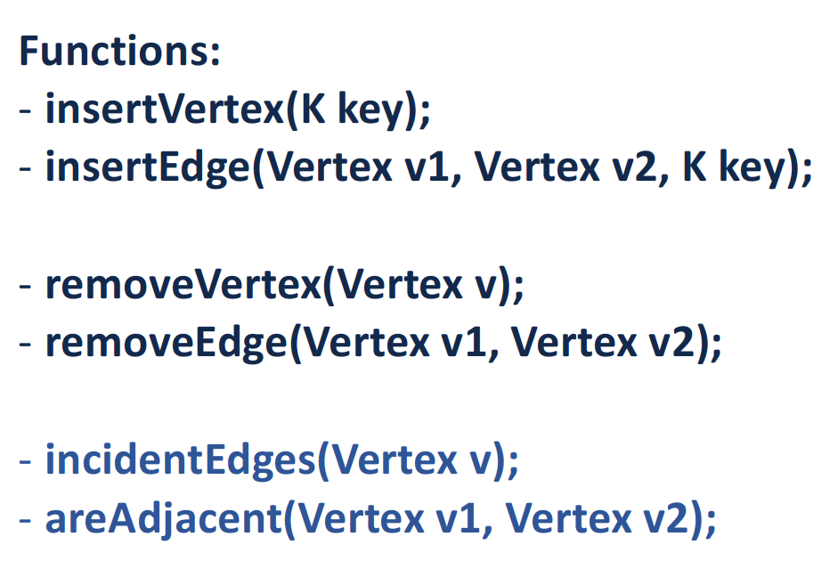
图的实现方法有很多,主要介绍以下三种:
- Edge List
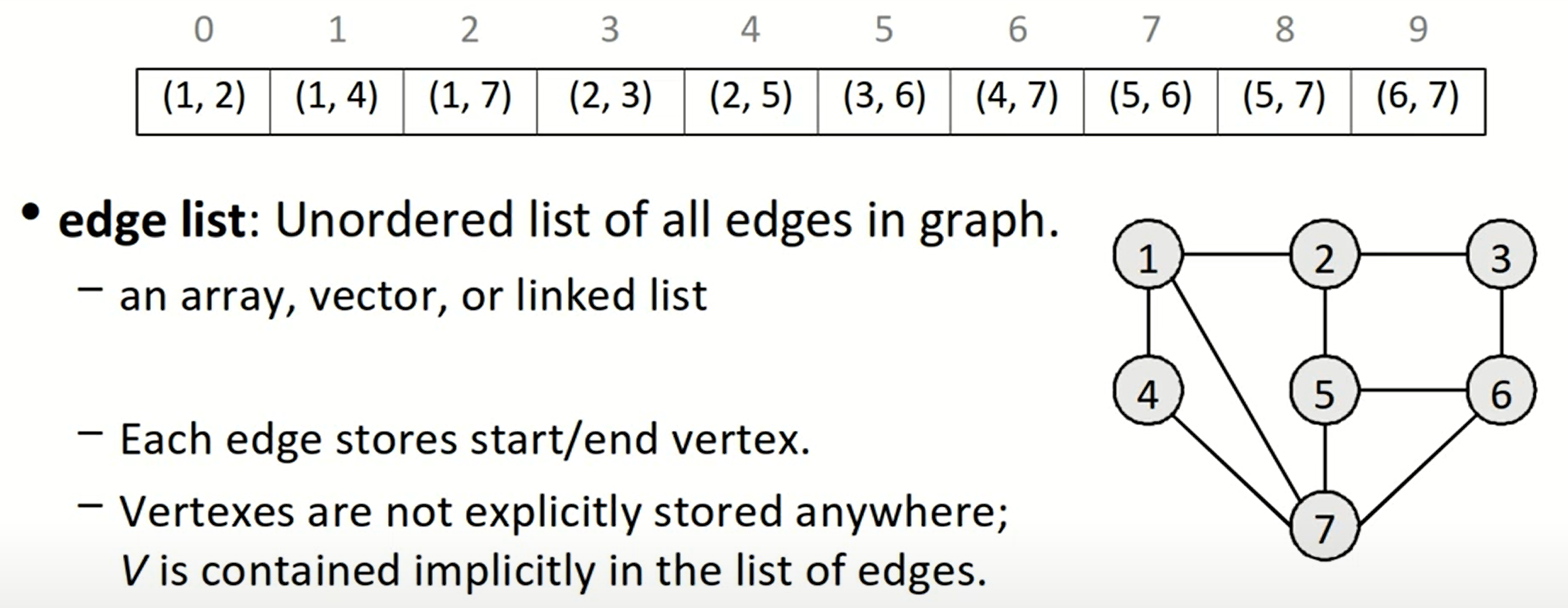
这是最基础的表示方式,使用vector<Edge>,或者set<Edge>,但由于性能表现不算好,所以使用的比较少。
- Adjacency Matrix
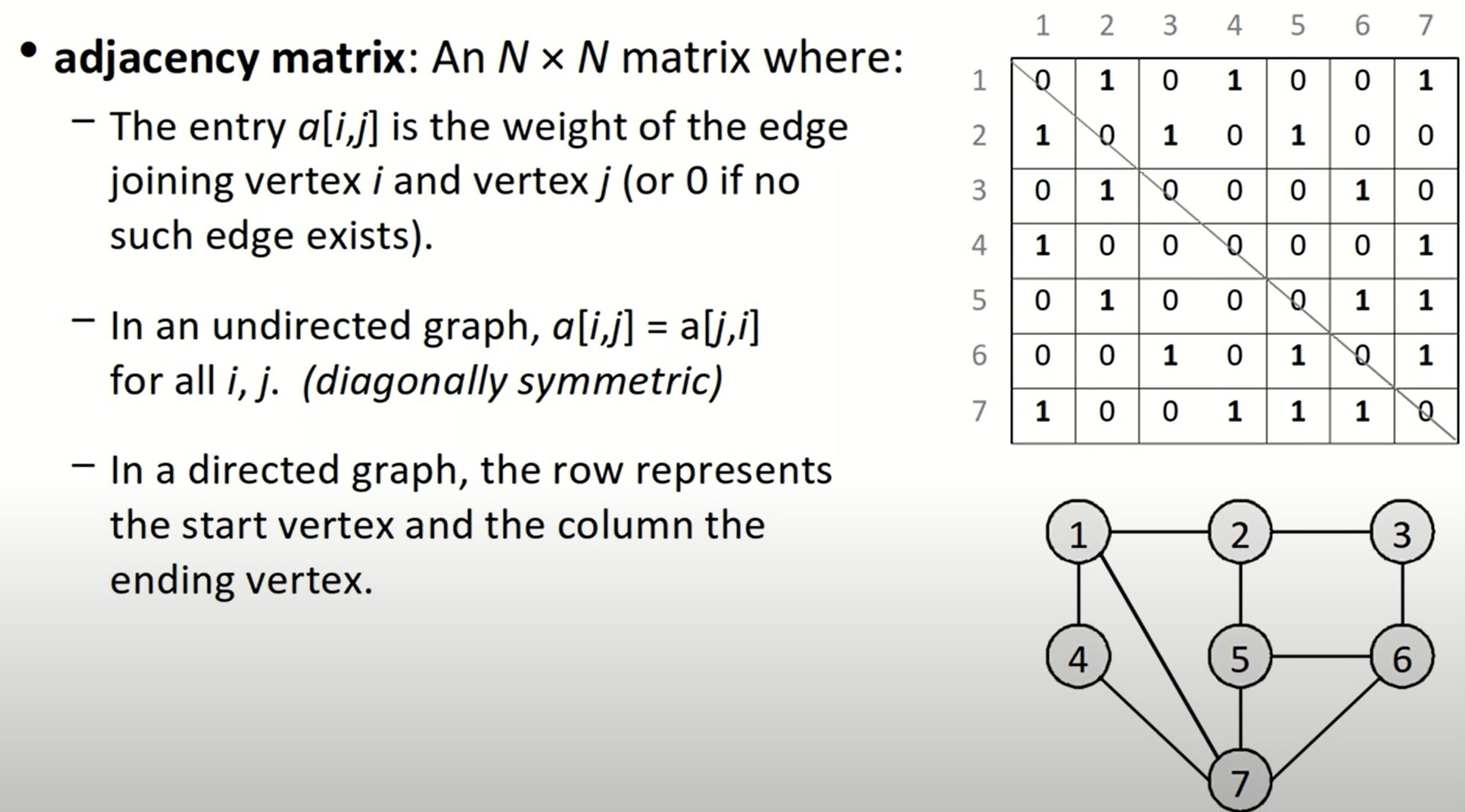
这种方法就是邻接矩阵,在邻接矩阵中,我们可以存储指向edge的指针,也可以存储bool值用于表示两个顶点是否邻接,或者存入边的权重,这取决于如何解决问题更加简捷方便。这种方法在插入或者删除节点时,因为需要改变邻接矩阵,所以时间复杂度为
。但是如果我们需要多次判断两个顶点是否互为adjacent,那么这种数据结构会是最高效的,因为此操作只需要常数级别的时间复杂度。
- Adjacency List
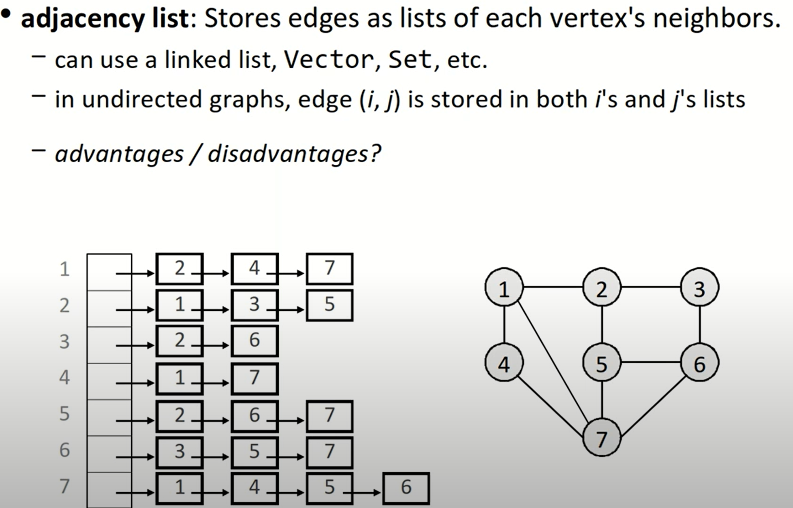
邻接表简而言之,就是在顶点表中的每一个顶点后,都跟上一组neighbors,代表了所有对于该顶点的indicent edges。这种图的表示方法应用较为广泛,我们可以使用stl中的list与pair来实现,也可以将整体结构视为一个map,值(邻接点集)为set,也即Map<Node, Set<Node>>.
这种方法的优点在于插入新的节点或者边,或者我们想找到某一个顶点的所有点邻接点;但是如果我们想解决类似topological sort的问题,或者查找边a->b是否存在,那么这可能需要我们遍历整个邻接表。
这三种设计各有千秋,最终我们可以得到如下的时间复杂度:
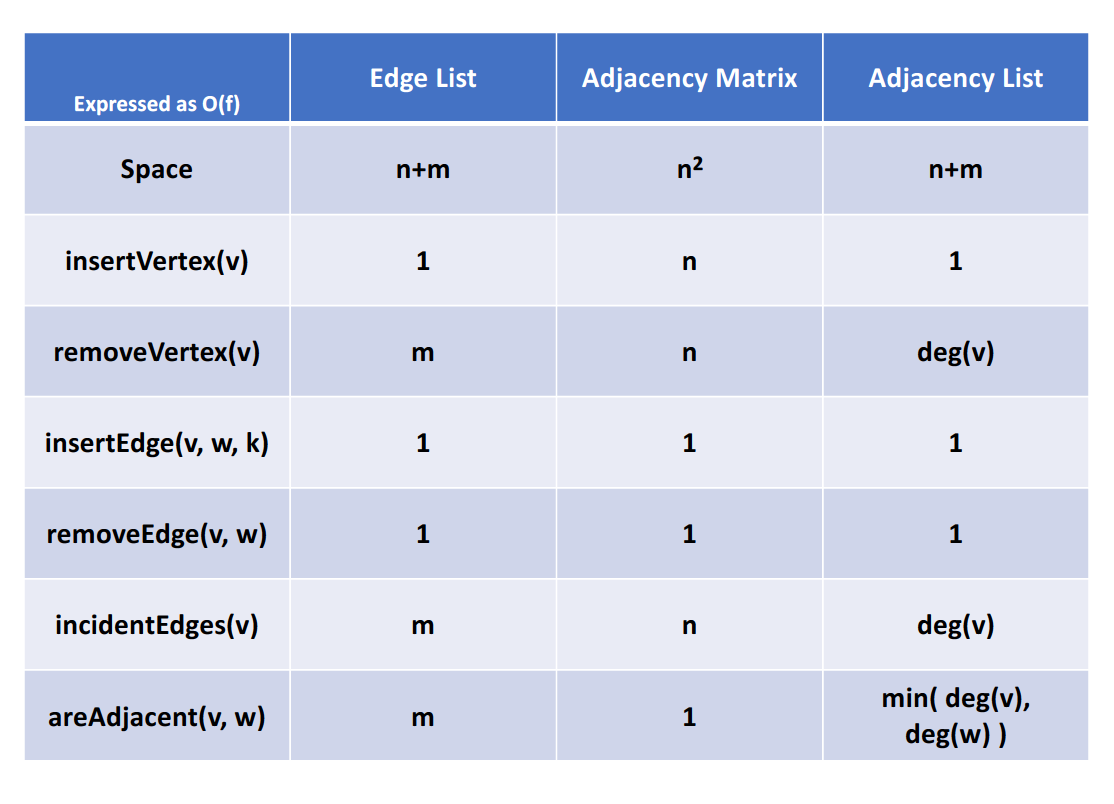
在实际实现中,主要关注邻接矩阵与邻接表。对于邻接表,其实我们可以表示成一个嵌套的vector的数据结构,其中的元素是指向顶点结构体的指针。对于有向图而言,邻接表只能表示出度,但是无法表示入度,所以我们在应对有向图时,常会使用逆邻接表的结构。而为了结合邻接表与逆邻接表,又开发了十字链表这一数据结构。
Graph Attribute
设无向图的顶点数为
$$n$$,边数为
$$m$$,经过证明,边数的范围是:
$$n-1 \le m \le n(n-1)/2$$Graph Traversal
图的遍历方法主要有BFS, DFS等。我们可能需要寻求任意路径、最短路径或者是最小代价路径。
关于深度优先搜索和广度优先搜索这两种算法,这两份伪代码描述的十分清晰:
DFS
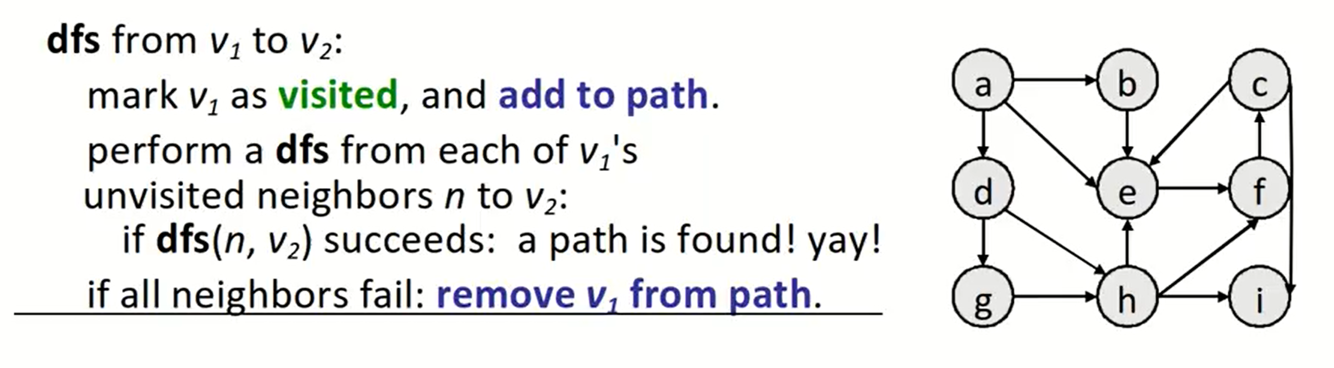
深度优先搜索常与回溯结合,我们首先沿着一条路径寻找下去,如果找到了就结束寻找,如果没有找到,我们就会自动回退到上一步。
BFS
BFS算法可以帮助我们找到两点之间的最短路径:
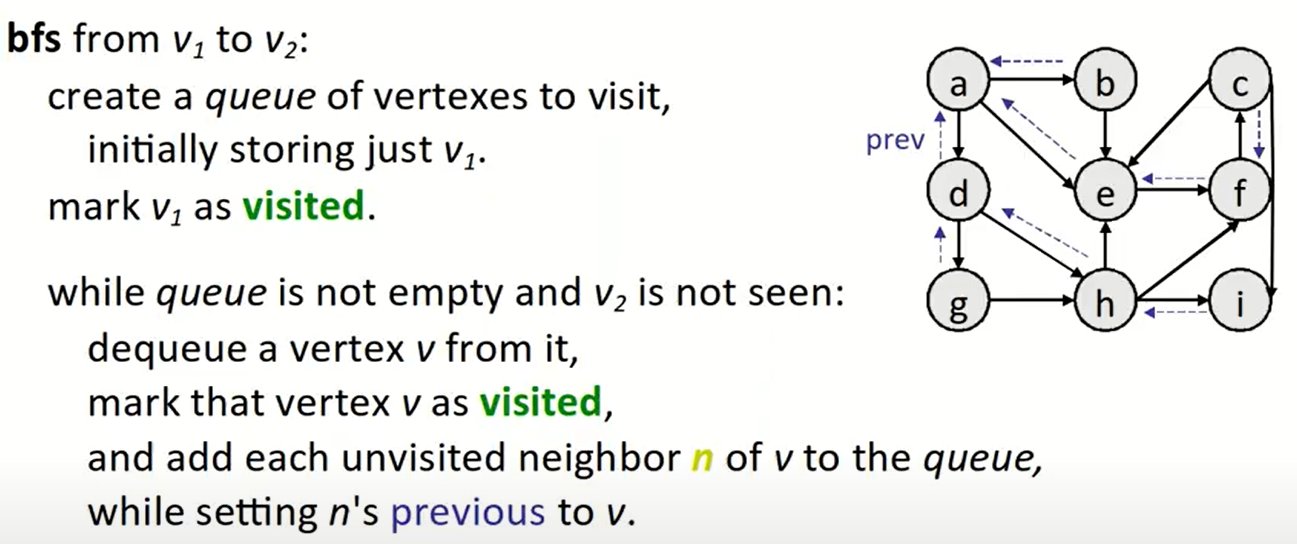
之前在树的DFS遍历与BFS遍历中也有类似的操作,这也说明了树其实就是一种特殊的图。BFS遍历需要借助堆栈或者队列来完成,在每一步中,先将当前队列出列,并将顶点标记为已访问;之后我们存储所有还没有访问过的当前顶点的邻接顶点进入队列(如果需要,则设置跟踪路径),直到我们找到目标点或者队列空了。
为什么BFS能够找到最短路径?因为使用的队列的数据结构,保证搜索深度每增加一层,所有的顶点都会被更新一遍
注意:
在所有的伪代码中,我们均把设置节点为已访问这一操作放到出列这一操作之后,但是在实际的代码编写过程中,我们更好的做法是把这一操作放在将neighbor入队列的后边;当我们在其还未出列时访问了该节点,那么不需要重复再向队列中添加它,此时!visited的判定条件可以帮助我们直接跳过。
Dijkstra’s Algorithm
此算法可以被视为BFS算法的升级版,如果所有路径的代价都一样,那么此算法将退化为BFS。
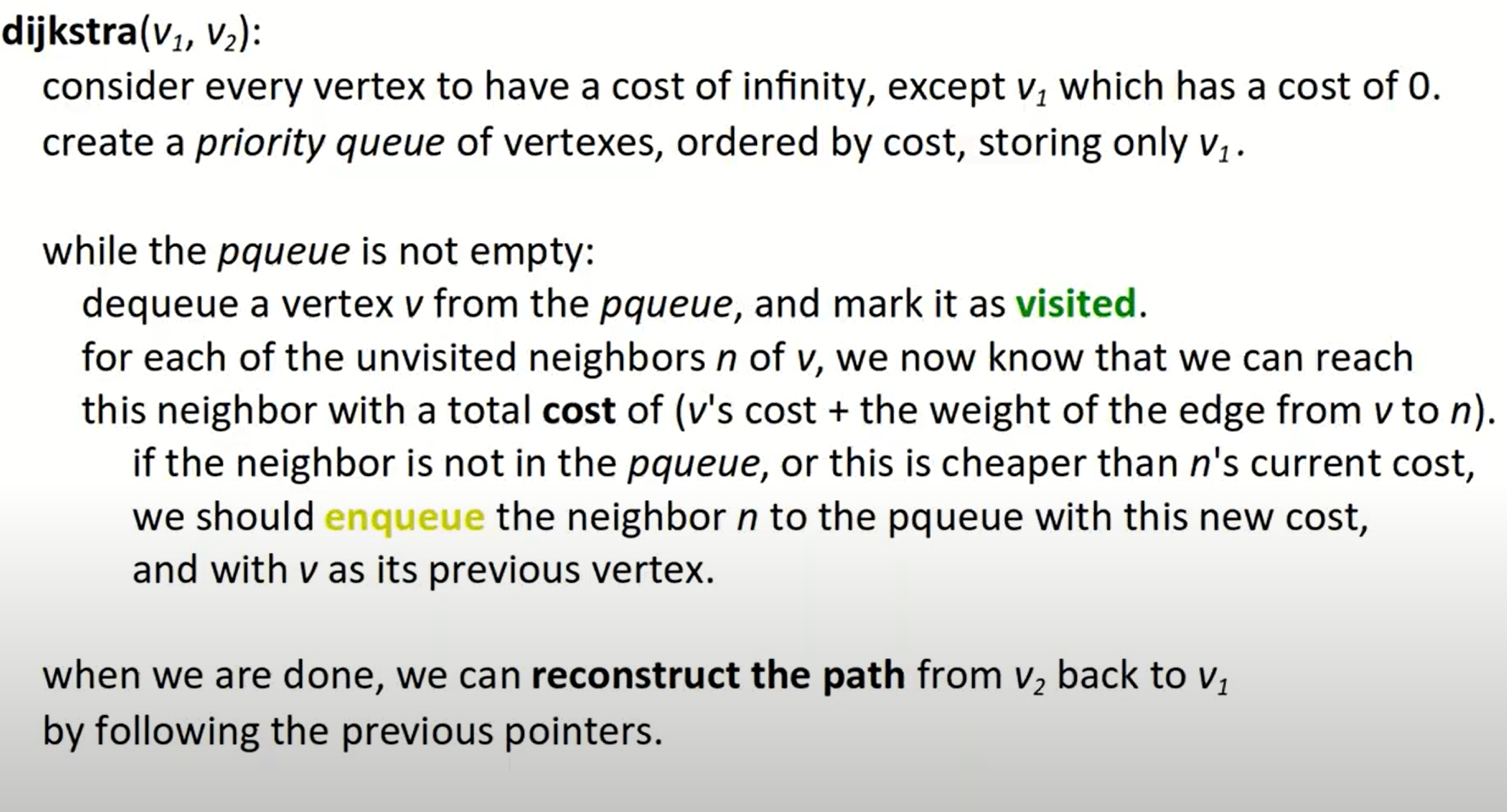
与BFS不同的是,这里我们使用的是优先级队列,且注意:
- 不能在找到要求节点时停止,这也是与BFS不同的一点,因为如果在找到节点时立刻停下,找到的路径未必是代价最小的,只有当此节点从队列中出列时,也即队列为空时,我们才会停止搜索过程。但是在迭代中,我们仍需要在将目标点出列后终止循环,而不能仅仅依赖于优先级队列非空这一条件,否则将会遍历过多的不必须节点。
- 如果某节点在此前的队列中存在,BFS会直接跳过该节点,但是dijkstra会判定优先级,从而决定是否更新此节点的优先级。
- dijkstra算法不适用于负数权重,我们可以这样理解:在算法执行过程中,我们只访问没被标记为visited的节点,就相当于默认了所有权重均为正数的条件(访问visited节点必然使得代价变大),而如果权重为负数,那么这显然是会发生错误的。
A* Algorithm
在dijkstra算法的基础上,我们加入启发式搜索的功能,所谓启发式搜索,也即尝试利用已有条件给算法一个大致的搜索方向,减少不必要的搜索过程。
admissible heuristic: One that never overestimates the distance.
- Okay if the heuristic underestimates sometimes
所谓admissible heuristic,是一个激进的启发方式,最终需要的代价大概率会比此代价大。正是依靠着这种功能,我们给搜索算法绘制了一个big picture。所以我们在每一步的代价变为:
基础的A*算法使用曼哈顿距离作为启发函数:
$$H(p_1, p_2) = abs(p_1.x - p_2.x) + abs(p_1.y - p_2.y)$$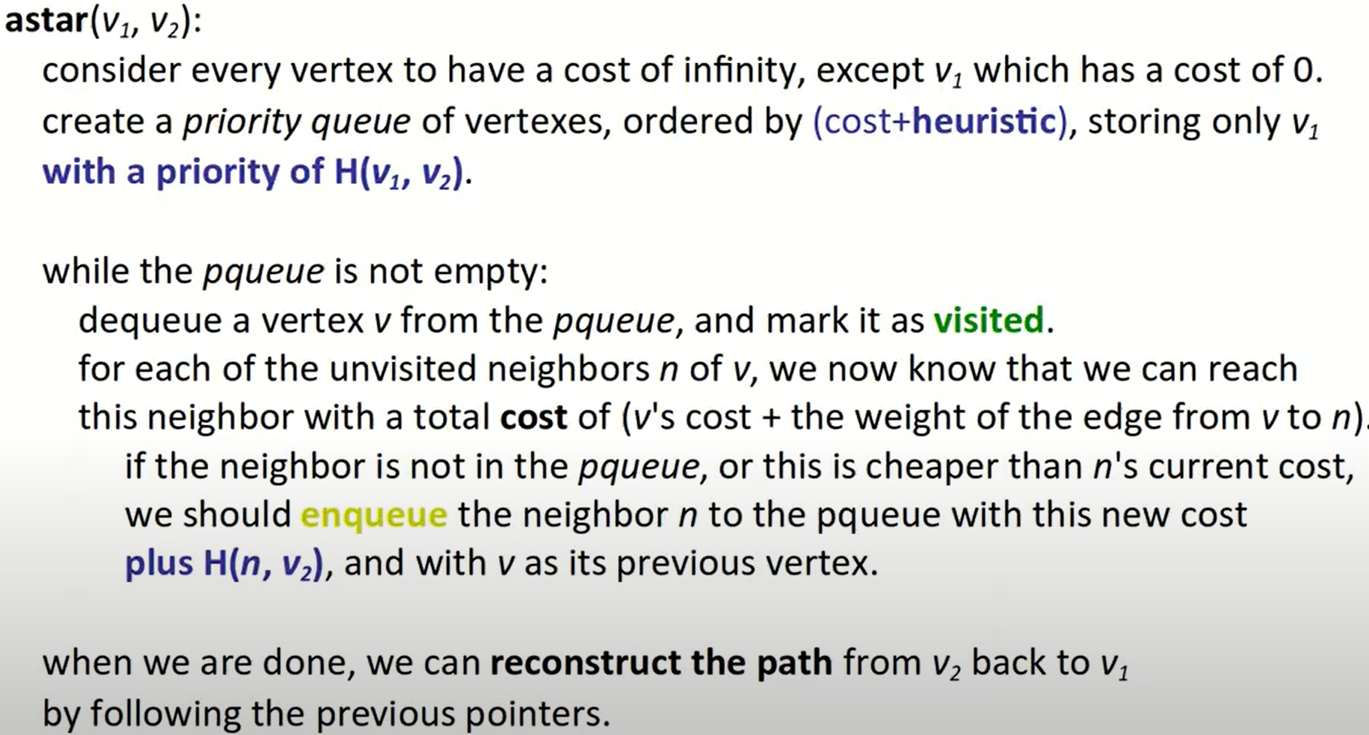
注意:
与dijkstra算法一样,当目标节点出列时,循环终止,同时我们要注意的一点是,优先级队列中的排序准则是cost+H(v1,v2),但是我们储存在已遍历节点上的cost不能添加启发函数,它仍然是preV's cost + edge's weight。**我们可以这样理解,优先级队列中加入启发式函数作为优先级的一部分,是给了搜索过程一个全局的观念,决定着哪些元素(节点)应当被首先搜索;而在具体的搜索过程中,我们不能够破坏具体的选择指标,即上一个节点的存储权重以及边的权重,这也是为什么一开始我们在出发点中存储了0,而非0+H(v1,v2)的原因。
Bidirectional search
一种替代A*算法的方式是双向搜索,也即从起点与终点分别同时开始搜索过程。
参照geeksforgeeks网站给出的实例程序,它包含了设计图类,邻接表设计,BFS设计以及最终双向搜索算法的实现, 我对代码进行了重构,放到我的Github仓库。
MST problem
什么是最小生成树?构造联通网的最小代价生成树成为最小生成树,MST问题的解决方法一般有两种,分别是Kruskal算法和Prim算法,这里只讨论前一种算法的设计。
Kruskal’s Algorithm
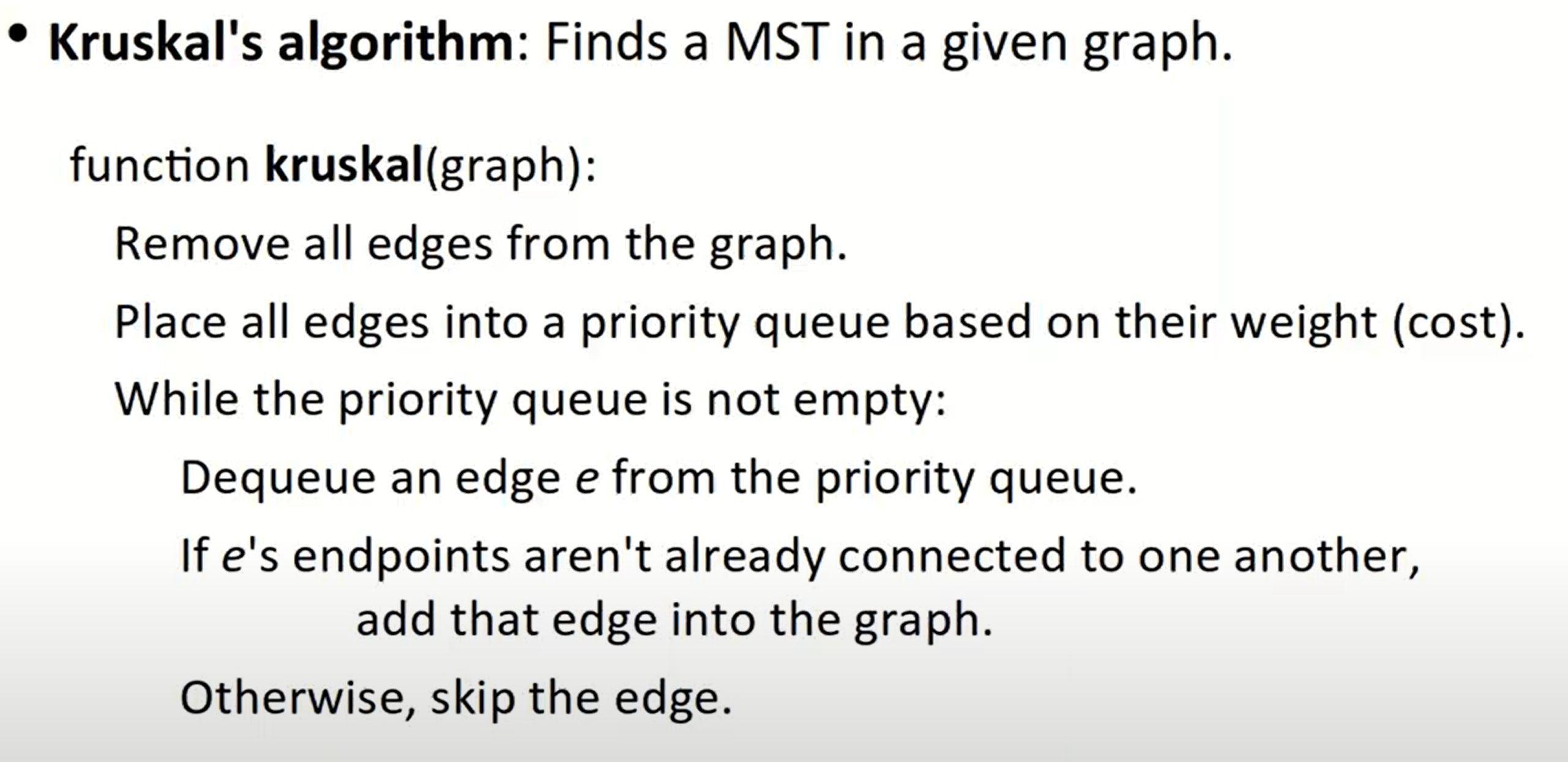
kruskal算法的使用与Union find紧密结合,所以首先解决一下Union find的问题。
Union find
这类算法来自于并查集–Disjoint Set,包含了查找与合并两种基础操作。无论遇到什么样的情景,我们都将问题抽象为几个独立的集合,存储元素均为整数,且所有元素均不重复出现。
- 对于查找操作,我们的核心思路是找到一个representative method,能够代表每一个独立的集合,如此一来我们就可以得到信息:所寻求的两个元素是否在同一个集合之内;
- 对于合并操作,我们最终的方案是使用一个upTree,并通过两种优化操作:path compression + smart union降低所需的时间复杂度。
并查集的时间复杂度的计算需要用到反阿克曼函数,特性是对于有限的操作次数n,时间复杂度为常数级别的,也即
$$O(1)$$.
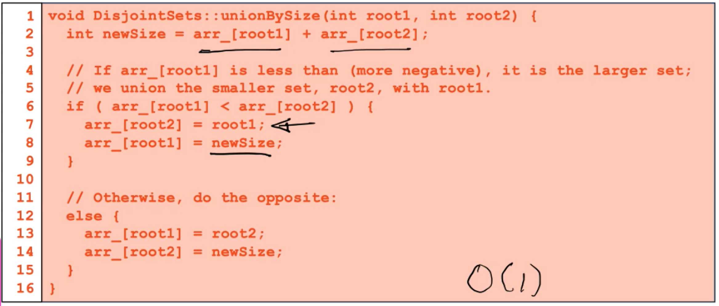
具体来说,对于每一个根节点,也即每一个独立子集的表示元素,在并查集中的存储值小于0,smart union的策略就是让这个根节点(的绝对值)存储这棵树的节点(元素)的个数。
另一种优化策略是根节点储存
$$-(h+1)$$,那么其效率将不如储存节点数高。因为当我们建好没有经过路径压缩的upTree后,查找操作的时间复杂度为
$$O(lgn)$$,按照高度合并的思路基于
keep the height of the tree as small as possible,而按照节点个数合并的思路基于minimize the number of nodes that increase in height,从概率上来讲,将节点数目少的树合并到节点数目多的树上是一种更划算的操作。
对于所有的非根节点,我们全部在对应的位置上存储其父节点的index,相当于一个指针,我们就可以顺着找到根节点的位置了。这样一来,如果两个位置上存储了同一个正数,也即数组中的某一个位置,那么此两节点必定位于同一个集合中,因为它们具有一样的表示元素。
需要注意,数组对于根节点和非根节点有着不同的含义.
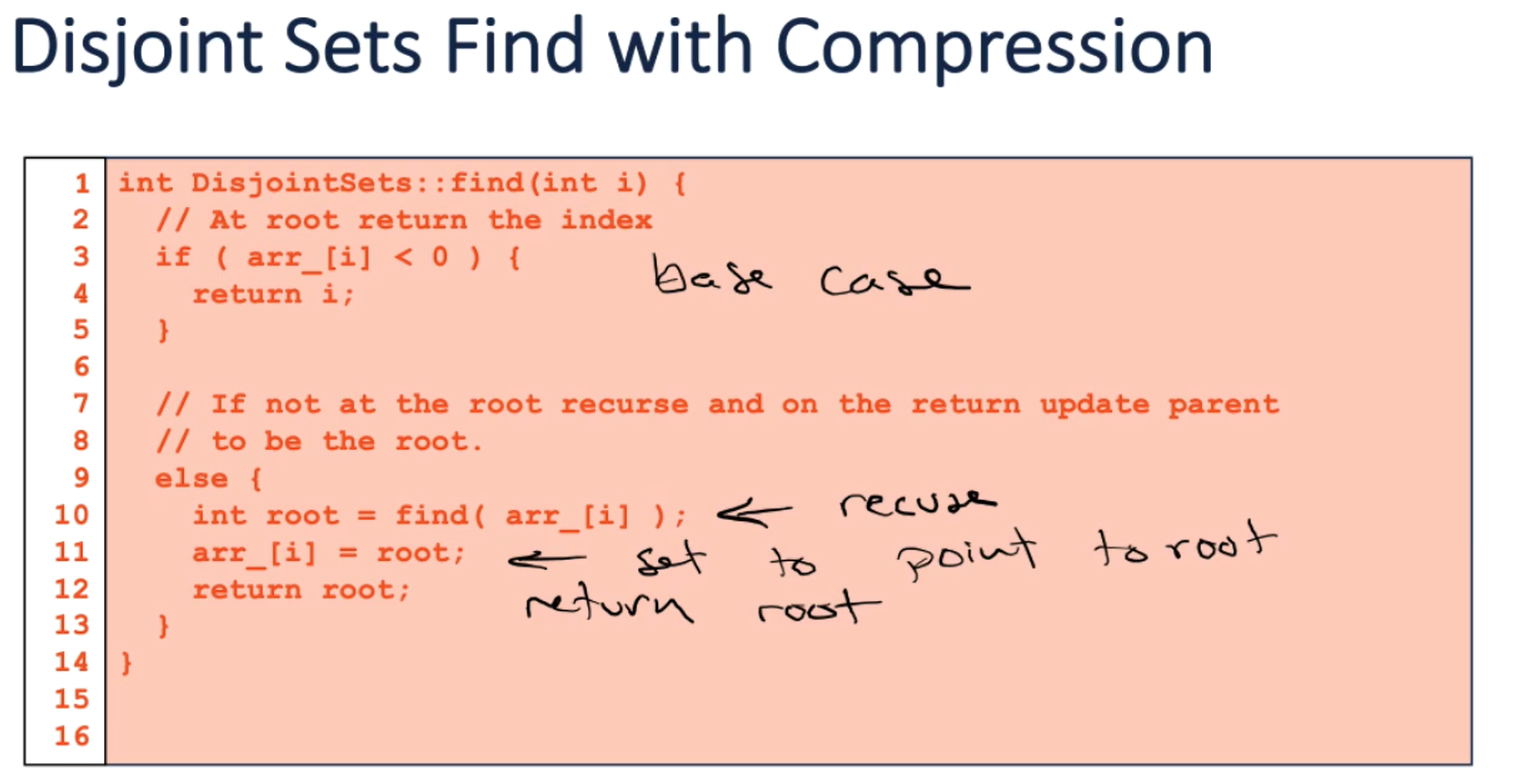
为了进一步减小时间复杂度,是用了路径压缩的技巧,这个做法基于如下思考:我们是否可以不用一直沿着树的节点向上、向上、向上找到根节点,再判定查找结果?我们想到,如果能够把树的子树全部展开,那么效果其实是一样的,但是展开之后我们就只需要往上找一层的父节点了:
现在回到Kruskal算法。我将一个demo放到了我的Github仓库.
所谓最小生成树,“最小”,是指代价最小,这是由优先级队列决定的;而“生成树”,则是由并查集决定的,为了说明这一点,我们可以试想一个最简单的图:三角形。其MST应当为两条边,当我们使用并查集时,如果前两条边均已被加入了并查集的forest,那么意味着并查集中[0,1],[1,2]位置的元素(顶点)都被放到了同一个集合中,具有相同的代表元素(根节点)。那么再次尝试[0,2]时,必定出现find(0) == find(2)的结果,所以第三条边不会被加入。
Union find用来查找图中cycle也是一样的道理。
所以在实现中,首先将所有点构建一个并查集,之后把所有的边加入到我们的优先级队列中,开始使用Union find寻找MST,只要两点还未被连接到一起就加入MST,当找到
$$n-1$$条边的时候停止(此性质之前说明过)。
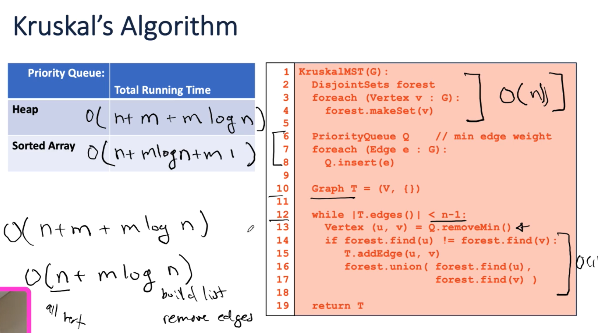
将步骤分解后,容易得到Kruskal算法的时间复杂度为
$$O(ElogV)$$,其中
$$E$$为边数,
$$V$$为顶点数。由于构建优先级队列有两种方法:使用sorted array或者heap。
- heap:如果图比较密集,或者说我们可能不需要去除所有边(堆的remove操作需要对数时间的复杂度)
- sorted array:在操作结束后仍保存着一个有序数组,这个结果可能对未来有用
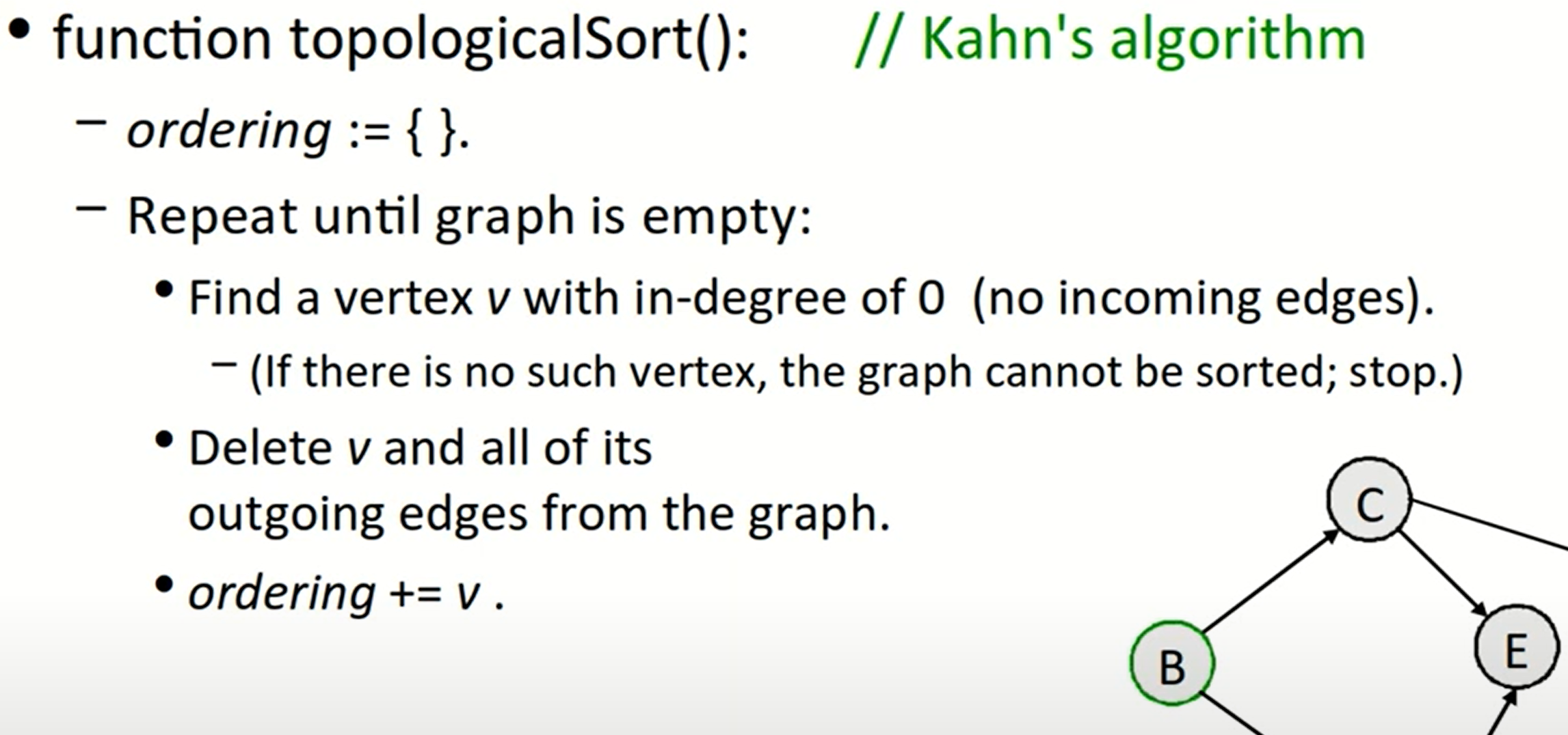
Topological Sort
拓扑排序的意义在于我们可以找到图中每个顶点的先后顺序,或者说哪些节点是另外一些节点的先决条件(比如可以用于寻找先修课程这类的)。该算法通过查找顶点的出度与入度实现。
注意这里讨论的对象是DAG,也即有向无环图。
Kahn’s Algorithm-O(V+E)
该算法简单来说,就是先找到入度为0的顶点(即不存在任何先决条件),此操作得以实现的理由是DAG不存在任何循环。之后将该节点以及与其相连的边全部从图中去掉,并将该节点加入vector中;重复以上过程:
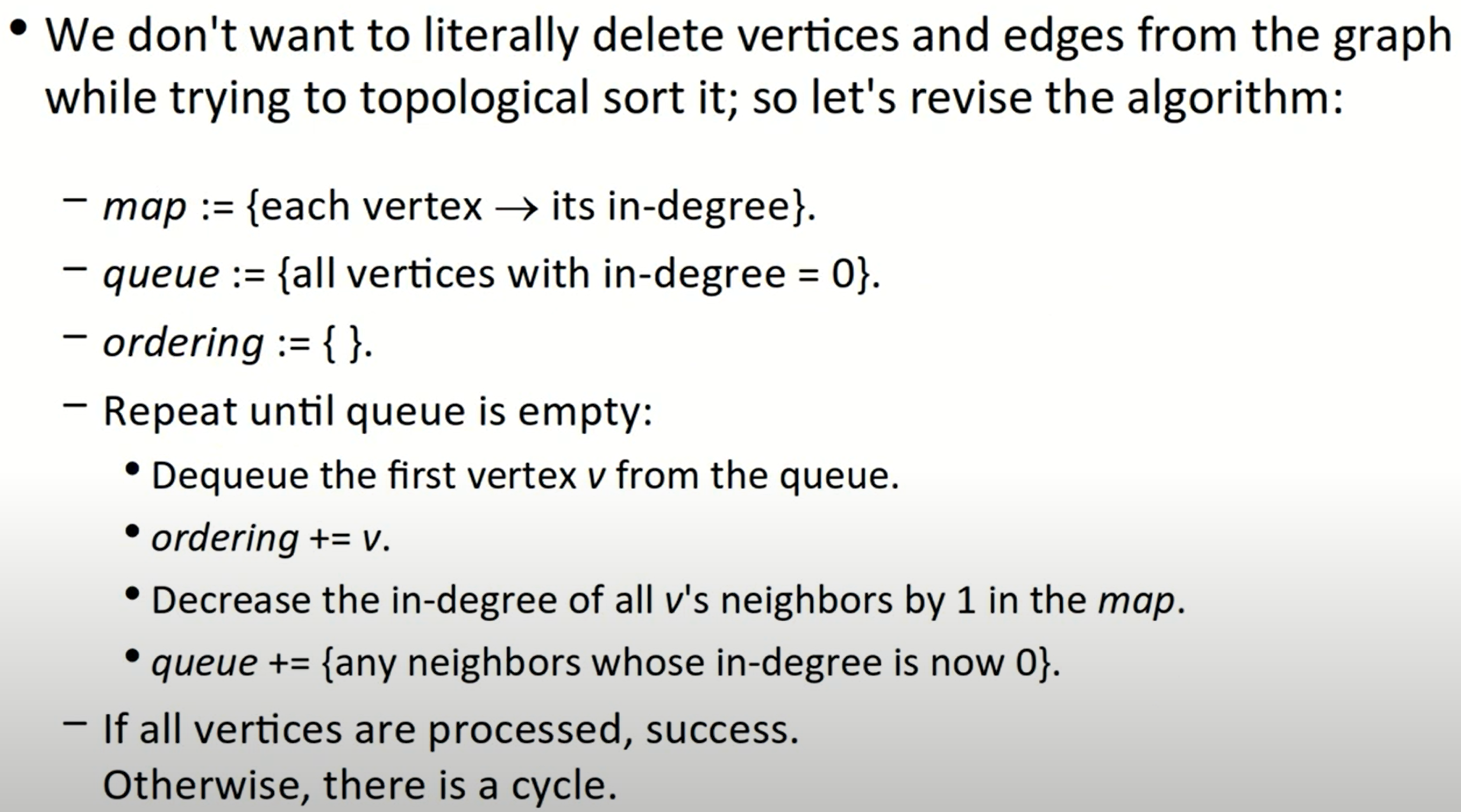
但在有时,我们可能不方便直接对图中的边与节点进行删除操作(或者复制操作),所以我们可以借助其他数据结构来完成:
Stanford CS 106X Lecture 25 – Hashing
散列技术是在记录的存储位置和它的关键字之间建立一个确定的对应关系
$$f$$,使得每个关键字对应一个存储位置
$$f(key)$$。我们将对应关系
$$f$$称为散列函数,也即Hash Function。他的输出被称为Hash Code;数据被存放在一段连续的存储空间中,被称为Hash Table。
一个足够好的哈希函数,可以使得我们的add, contains, remove操作的时间复杂度均被控制在
。散列函数的设计原则是使得整个散列表的数据存储越分散越好。
Probing
常用的一种方法是除数留余法。一个很大的质数会帮助我们将数据变得分散。在操作过程中,可能会出现很多冲突(collision),为了解决这个问题,我们会使用probing,可能是线性的(线性探测),也可能是二次幂的(二次探测):
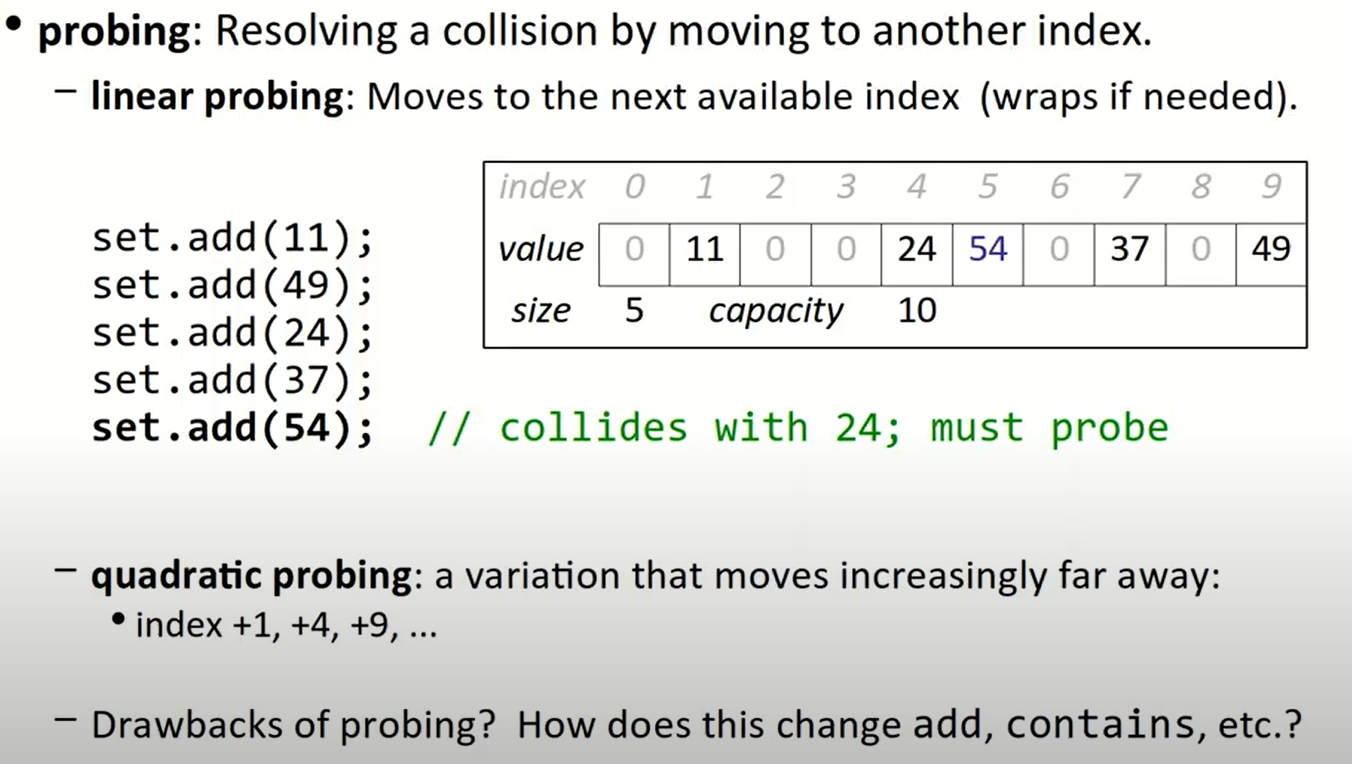
但是这些探查方法可能会形成一些clusters(堆积),在相邻的多个点位内均存放着数据:

这意味着我们需要循环探测在这些小集合中是否存在我们需要的数据,直到我们遇到了0,或者设置的特殊结束标志位,再到下一个可能的存储位置继续检测,显然会大大降低我们的效率。
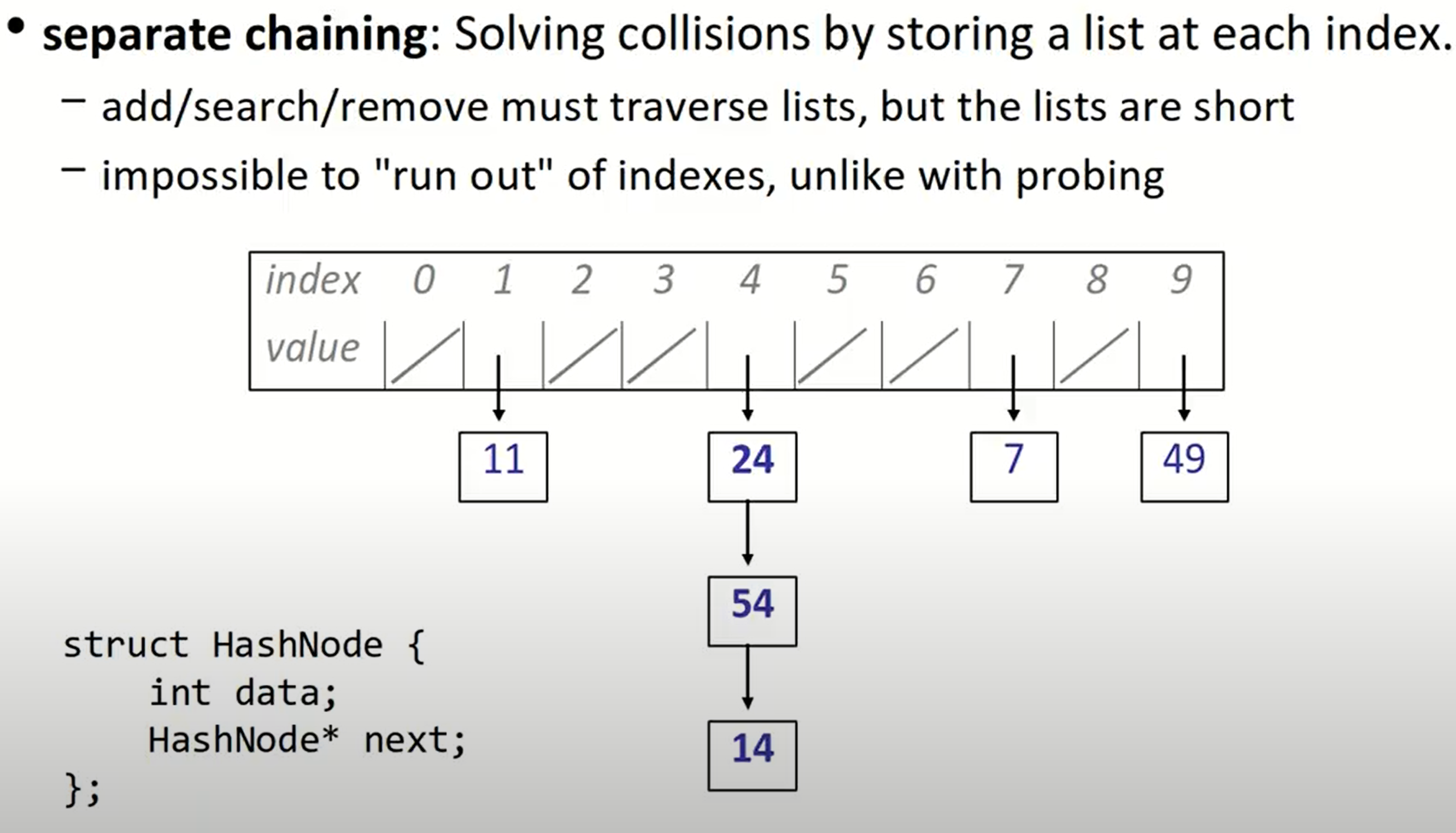
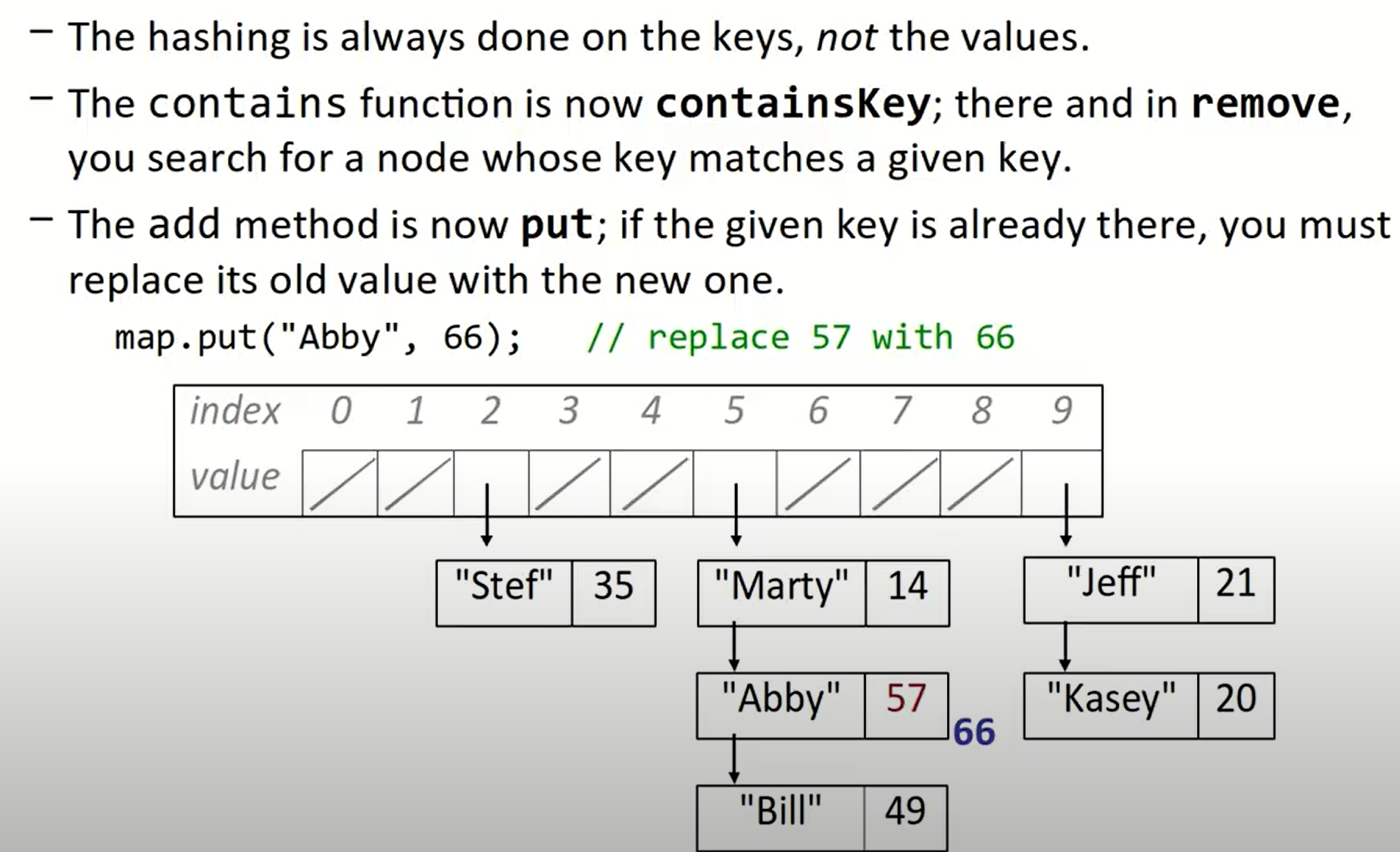
Separate chaining
另一种解决冲突的方法是separate chaining,也叫链地址法。每一个位置里都存储着一个单链表,所以地址不可能被耗尽,但是这降低我们对数据的操作效率。
Rehashing
我们也可以在散列表填充到一定程度(load factor = (# of elements) / (hash table length))后扩张散列表,但是需要注意的是,我们不能简单的将数据复制到新表的原坐标中,因为使用除数留余法,我们需要重新根据数组的长度对数据进行排列。
Rehashing with separate chaining
使用separate chaining時進行rehashing的例子:
// previous array:
using ValueType = std::pair<const K, M>;
struct node {
    // it's a pair
    ValueType value;
    node* next;
    // constructor...
}
vector<node*> buckets_array;
// the new array
vector<node*> new_bucket_array;
这个问题应当怎么去思考?首先我们想他应当有两层循环,外层用于遍历array,内层用于遍历每一个link list并将其重新hash:
for (auto& curr : bucket_array) {
    while (curr != nullptr) {
        // do something
    }
}
接下来,我们要如何把链表中对应的节点重新分布到新的表中呢?
我们想,无论如何,是会有如下的语句的:
// calculate the hash value:
const auto& [key, mapped] = curr->value;
int index = _hash_function(key) % new_bucket_count;
并且我们一定会利用index做这一步(类似地),来把一个数据(指针)复制到我们的新表中:
new_bucket_array[index] = curr;
可是现在问题变得棘手,我们每一个格子里,不可能一直都只存放一个指针,而是要存放一个链表,当我们这一次把格子中的数据更新为这个指针时,下一次又有一个数据有了相同的哈希值,我们该咋办呢?
假定新表中格子A处目前存放了指针ptr1,我们经过计算后想要把旧表中的ptr2也放到A里,那么显然此时有两种做法:
- 把
ptr2连接到ptr1后边 - 把
ptr1连接到ptr2后边
对于方案1,格子A的起始值始终是ptr1,这相当于链表的尾插法,意味着每次我们都要遍历到A格的链表的最后来插入新数据;
而方案2是头插法,显然我们只需要调整几个指针位置–先把ptr1连接到ptr2,再把当前ptr1所在的A格子里的位置腾给ptr2,就可以实现插入操作,故2是效率更高的选择,我们尝试写出代码:
curr->next = new_bucket_array[index];
new_bucket_array[index] = curr;
// go forward
curr = curr->next;
但显而易见的是,我们需要一个temp指针来记录指针当前位置,否则一切都错乱了!同时我们也要留心curr=curr->next这条语句的位置,因为对temp->next赋值这个操作相当于切断了temp指针原本的通路,把temp即我们前述的ptr2指针和ptr1给连起来了:
auto temp = curr;
curr = temp->next;
temp->next = new_bucket_array[index];
new_bucket_array[index] = temp;
最后,yi所有旧表内的指针都被我们链接并转移到了新表中,我们可以用std::move操作来将新的vector赋值给旧的类成员vector:
for (auto& curr : bucket_array) {
    while (curr != nullptr) {
        const auto& [key, mapped] = curr->value;
        int index = _hash_function(key) % new_bucket_count;
        auto temp = curr;
        curr = temp->next;
        temp->next = new_bucket_array[index];
        new_bucket_array[index] = temp;
    }
}
bucket_array = std::move(new_bucket_array);
另一个值得注意的点,是这段代码中的引用使用问题,如果我们不想更改类本身,则在for循环处不要使用引用传递,而在这里,传递引用之后进行curr=temp->next的操作正是我们想要的,我们想要将旧表中A格的第一个元素替换掉。
Good hashCode behavior
Consistency with itself
hasCode(x) = hashCode(x)
Consistency with equality
a == b –> hashCode(a) == hashCode(b)
a != b -/> hasCode(a) == hashCode(b)
Good distribution of hash codes
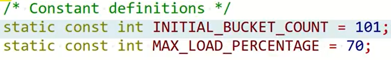
Possible hashCode (for strings)
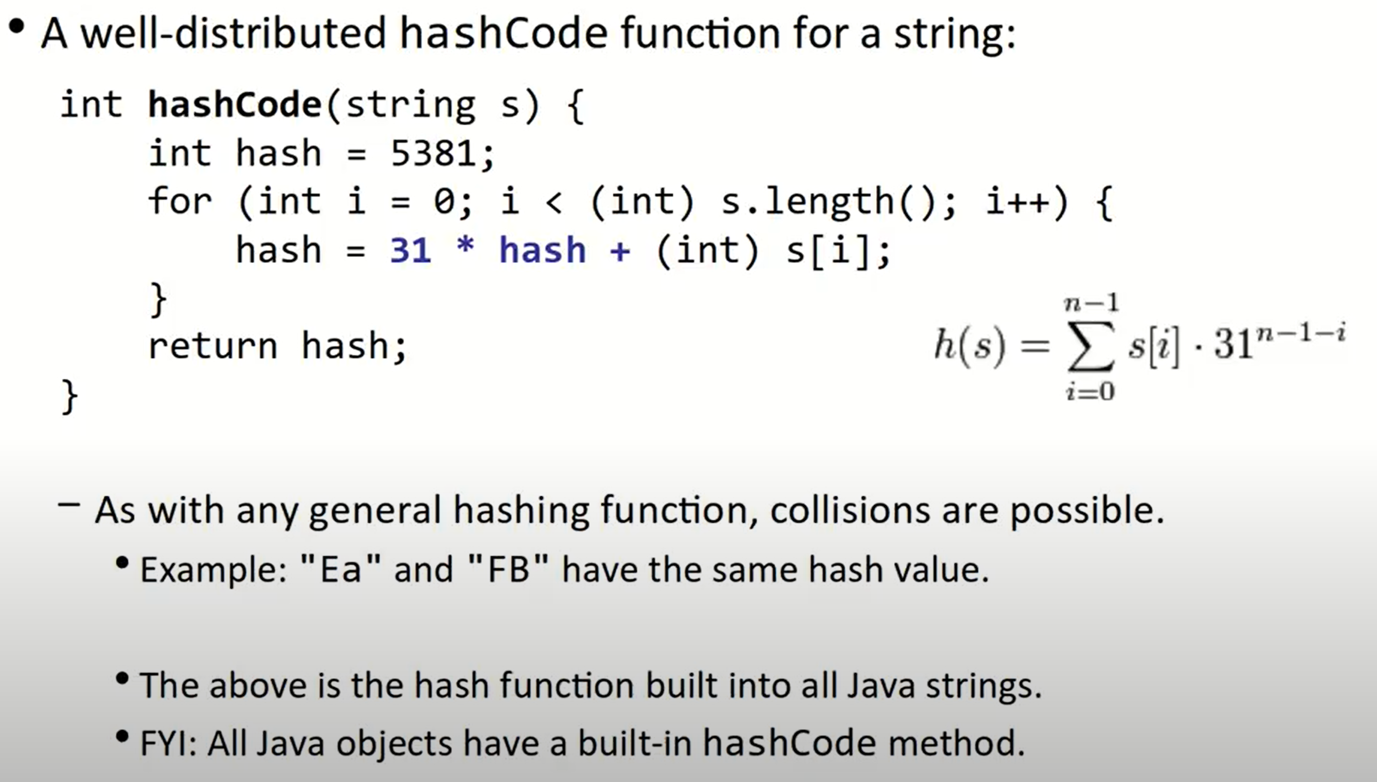
JAVA内置的算法
hashSet & hashMap
Stanford CS 106X Lecture 26-27 – Inheritance & Composition & Polymorphism
Inheritance
call super class constructor
SubclassName::SubclassName(params)
    : SuperclassName(params) {
        statements;
    }
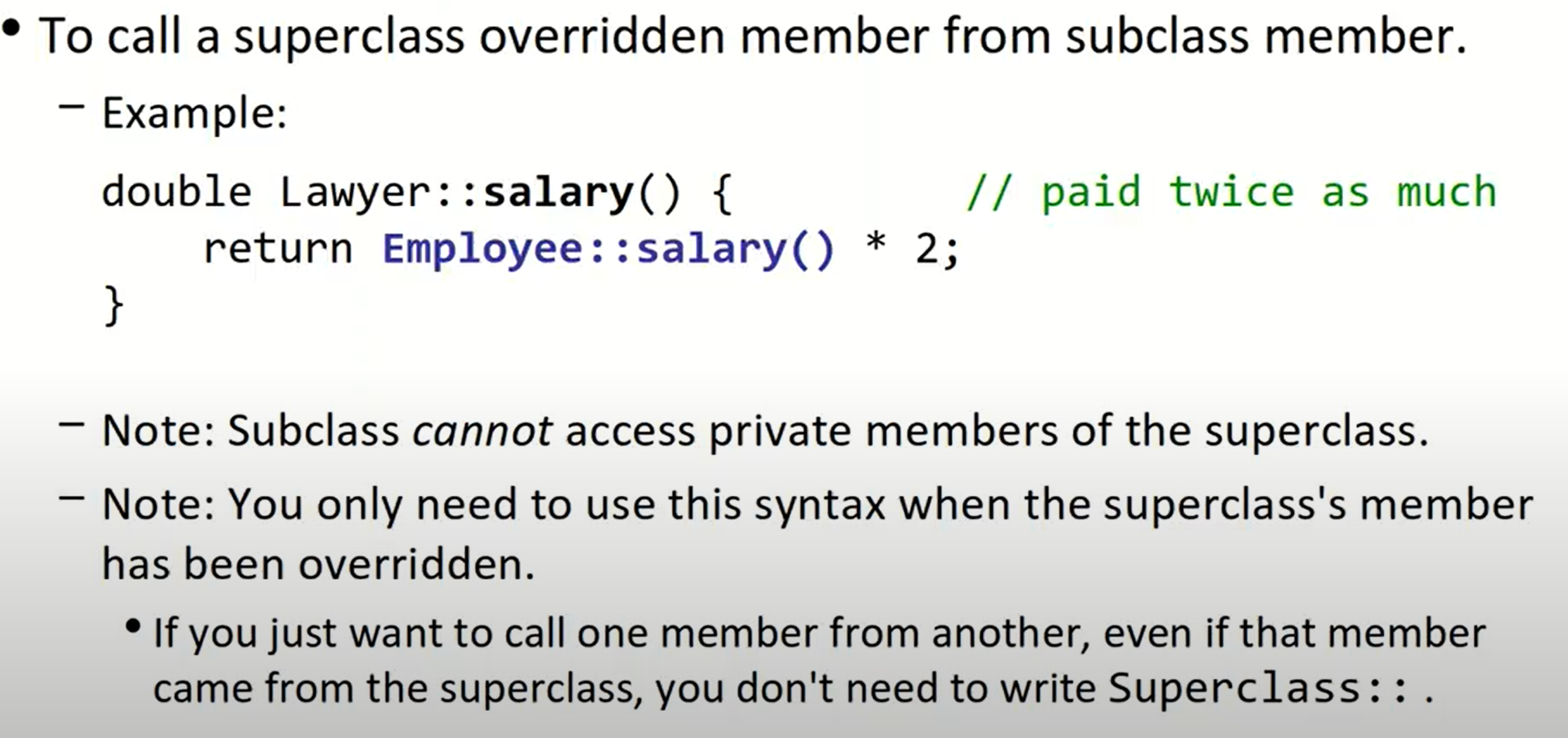
call superclass member
private inheritance
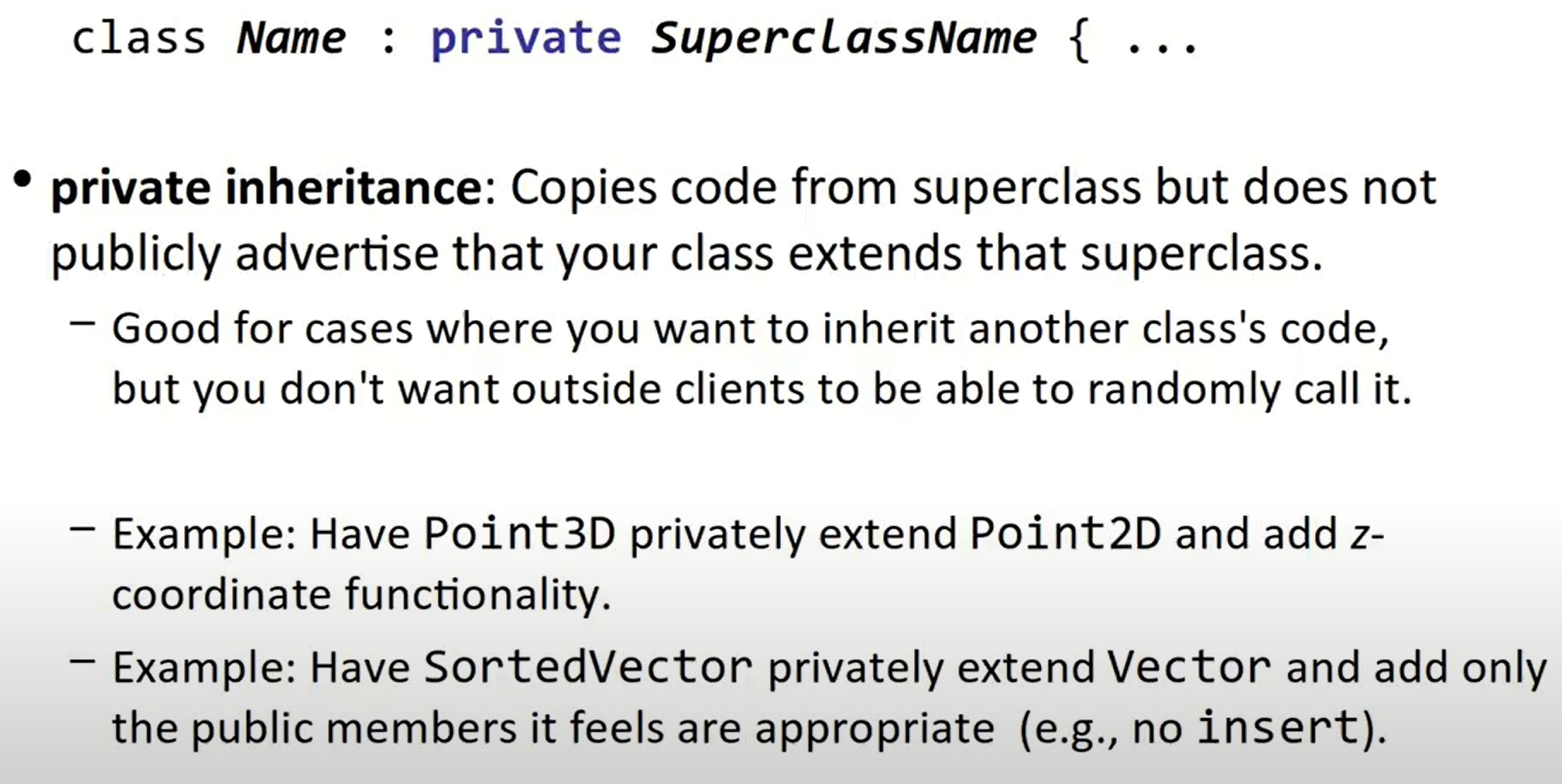
这个操作简而言之,就是在类外部,我们无法得知两者是继承的关系。
pure virtual functions
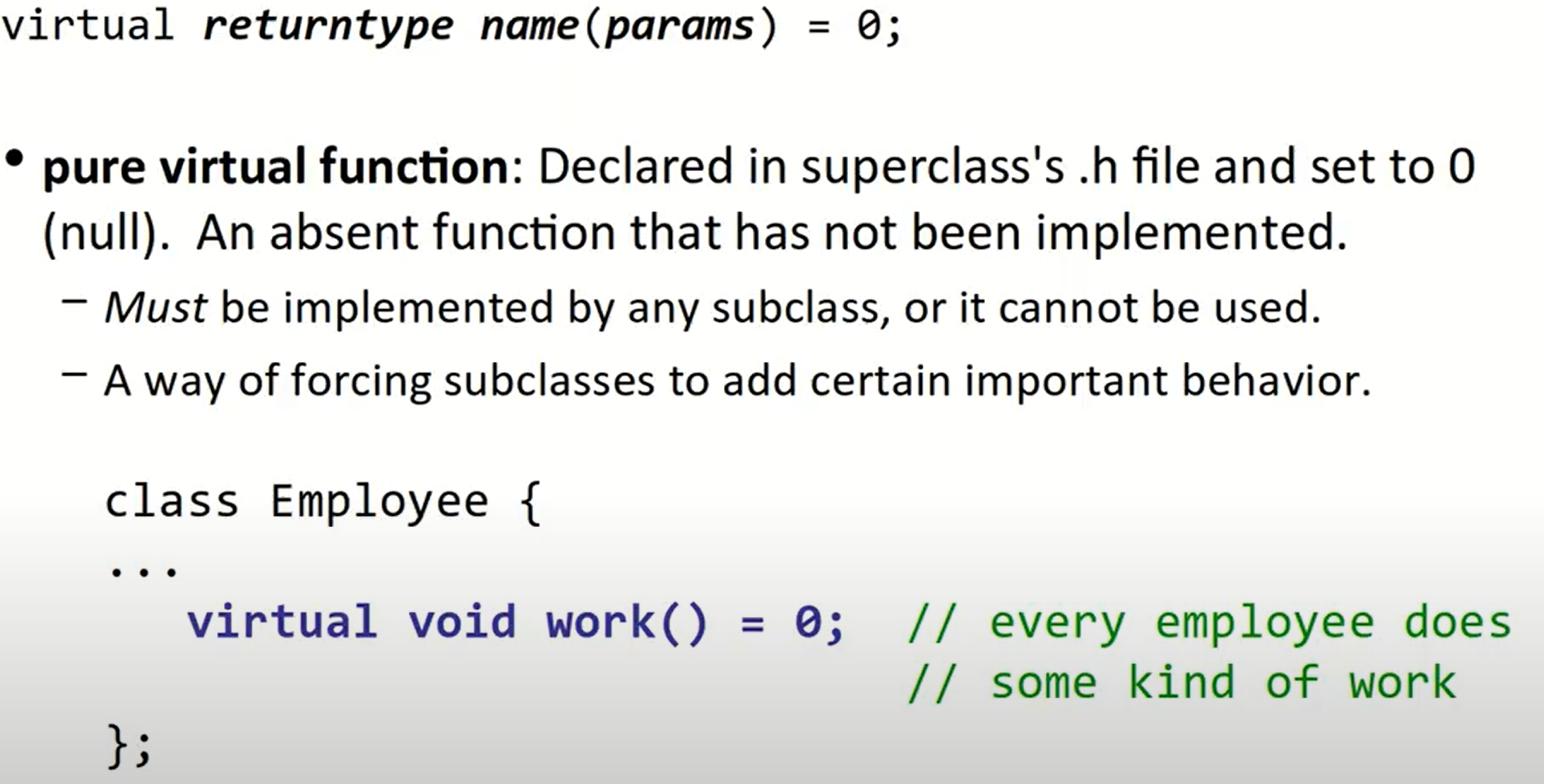
对于virtual关键字,我们需要注意:如果想继承某个函数,我们可以不加该关键字,程序可以正常编译,新的继承函数也可以编译通过,但这会导致程序在运行时不知道去调用新的继承函数(缺少了动态绑定的过程)。
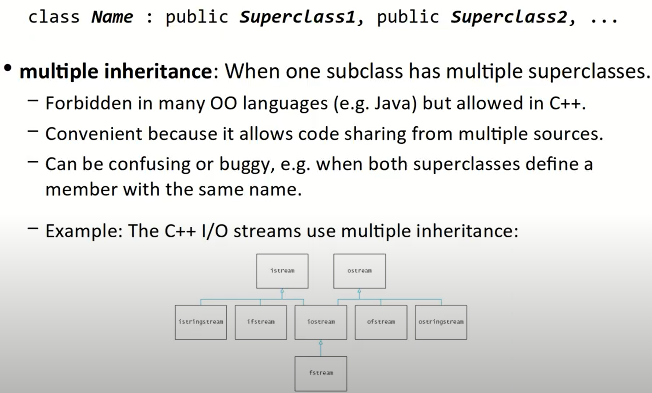
multiple inheritance
Polymorphism
Polymorphism is the the ability for the same code to be used with different types of objects and behave differently with each.
For example, even if you have a pointer to a superclass, if you call a method that a subclass overrides, it will call the subclass’s implementation.
Polymorphism is important because for instance by default, with a vector of the same type of object, you might expect that calling a method on all of them would execute the exact same code.
Polymorphism means that is not true!
With templates, we create one class that works with any type parameter. At compile-time, C++ generates a version of this class for each type it will be used with. This is called compile-time polymorphism.
With inheritance, we create multiple classes that inherit and override behavior from each other. C++ instead figures it out at runtime using a virtual table of methods. This is called run-time polymorphism.
mystery problem
对于如下的继承关系:
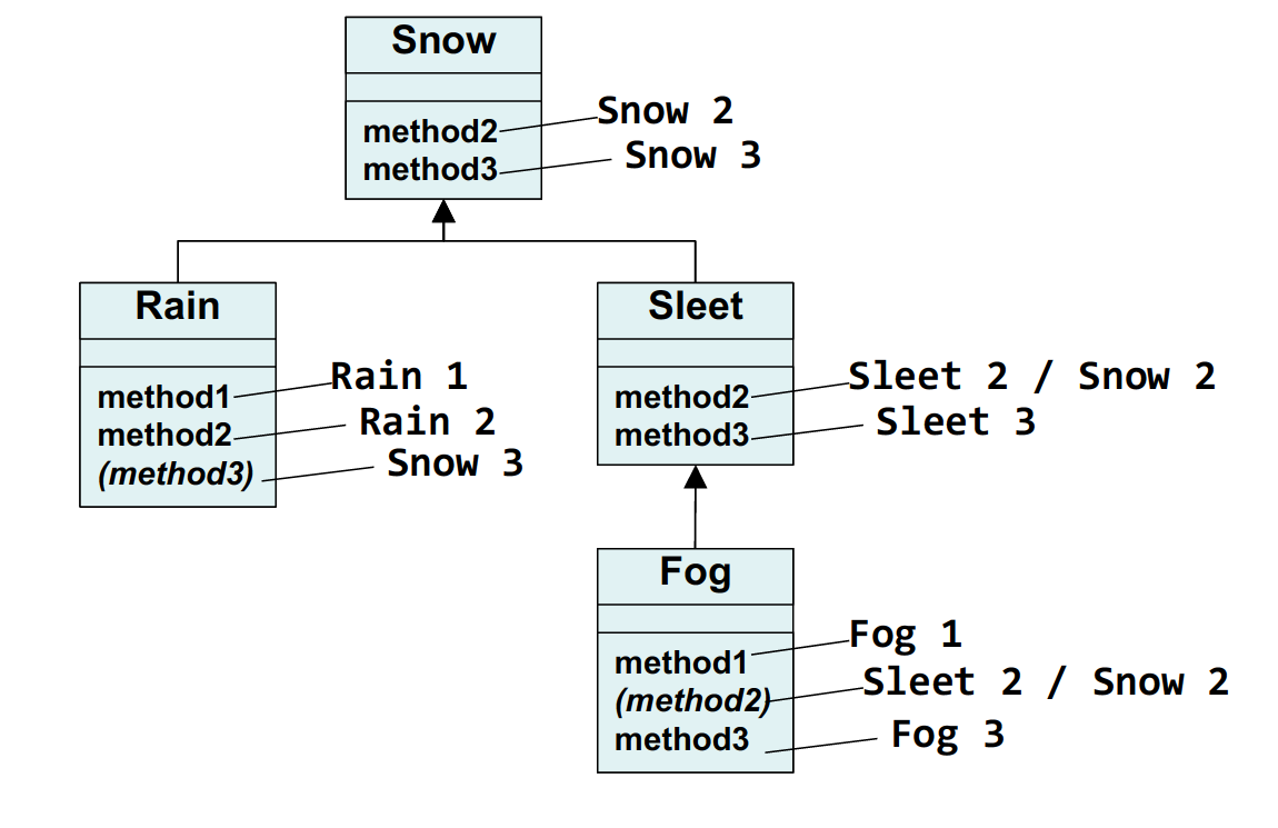
我们讨论第一种情况:
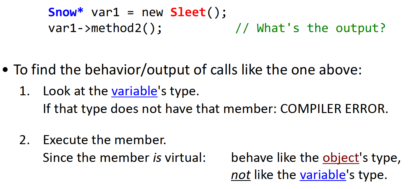
也即在编译时,我们需要看变量类型是否包含此方法,但是在执行该成员函数时,我们执行的是对象类型中的该成员函数。Ploymorphism: 如果object type中没有找到这种成员函数,那么类似于CS 61A中python不断向上寻找parent frame的方法类似,C++也会继续尝试在基类、基类的基类中寻找该成员函数,直到第一次遇到它。需要注意的是,如果在基类的A方法中调用某个方法B,而没有使用::标记,那么当编译器找到并执行parent frame中的A方法并执行到B处时,因为成员函数传入的仍然是派生类对象的地址,会首先回到派生类定义处,尝试执行方法B,如果带了::标记,那么编译器会直接到对应的类中开始寻找,并重复上述过程。
第二种情况:(类型转换)
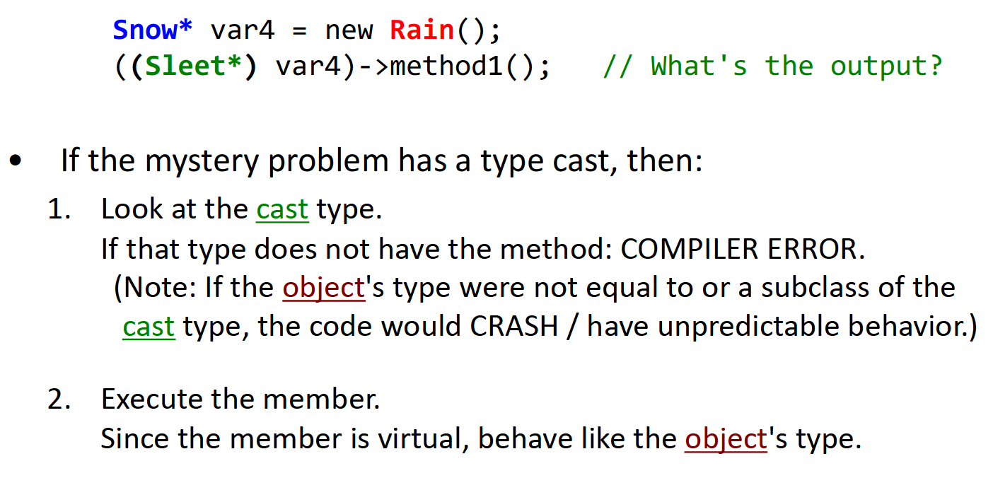
与第一种情况类似,在编译时我们查看的是左侧变量的类型,也即类型转换之后的类型,但是在运行时,指向的是object的成员函数。
同时需要注意,object类型不能是cast类型的基类。也就是说,这种转换方法只能做向上类型转换,当向上强制类型转换出现时,原派生类的对象内容被切割(object slicing)。反过来,如果是基类想要强制转换为派生类,将会崩溃或者产生未定义行为。
Stanford CS 106X Lecture 26 – Sorting
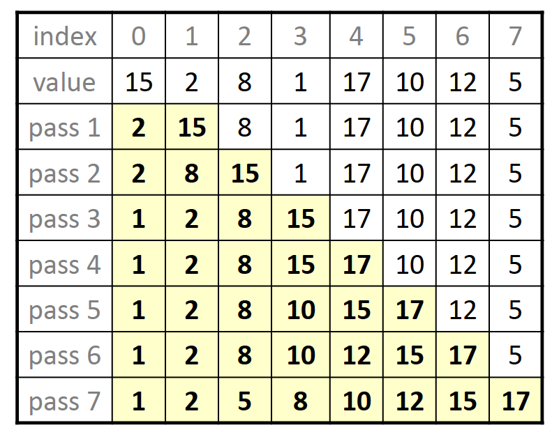
稳定:如果原数组中相同大小的两个数据在排序前后的位置关系不发生改变,那么称这种排序算法是稳定的。
selection sort-$$O(n^2)$$+不稳定
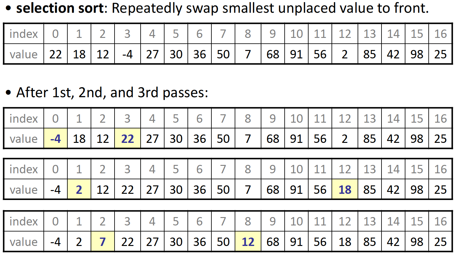
基本思路是逐渐扩展已经排序好的sublist,每次在之后的序列中找到最小的数据的位置,并将其与起点数据交换:
void selectionSort(vector<int>& v) {
    for (int i = 0; i < v.size(); ++i) {
        // we need to find the smallest index
        int minIndex = i;
        for (int j = i + 1; j < v.size(); ++j) {
            // find the index of smallest remaining value
            if (v[j] < v[minIndex]) {
                minIndex = j;
            }
        }
        // swap the smallest value to proper place -- v[i]
        swap(v[i], v[minIndex]);
    }
}
insertion sort-$$O(n^2)$$+稳定
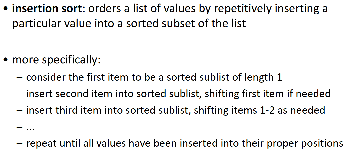
与选择排序的思路相反,插入排序是直接选择后边一位的数据,并尝试在前边的有序数组中插入到合适的位置,如果我们对比选择排序与插入排序的代码,这两者其实是十分类似的:
void insertSort(vector<int>& v) {
    for (int i = 0; i < v.size(); ++i) {
        // we need to keep the current value
        int temp = v[i];
        // slide elements to make room for v[i]
        int j = i;
        while (j >= 1 && v[j - 1] > temp) {
            v[j] = v[j - 1];
            j--;
        }
        v[j] = temp;
    }
}
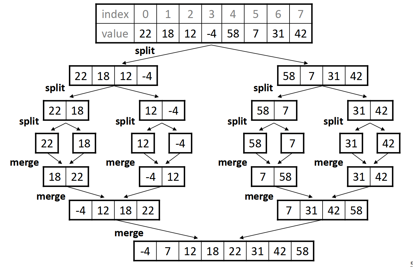
merge sort-$$O(nlogn)$$+稳定
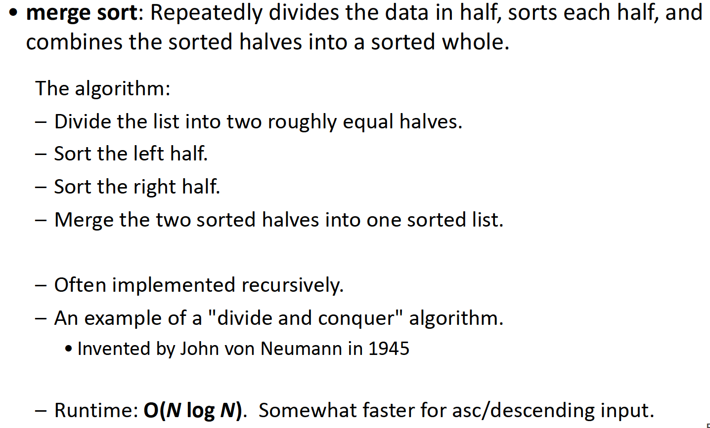
归并排序将数组分为两半,分别对两半进行排序,之后再把已经排序好的两个子数组组合在一起(merge)。这一过程可用如下图表示:
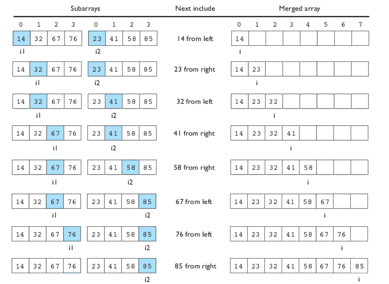
merge操作是归并排序中一个较为复杂的部分,其实并不难理解,主要过程就是使用类似于双指针的想法,逐步探查两个子数组各自的元素,按顺序将他们合并到一起:
vector<int> tmp(v.size());
void mergeSort(vector<int>& v, int l, int r) {
    // base case
    if (l >= r) return;

    // 确定分界点:
    int mid = l + r >> 1;

    // 递归两半边:
    mergeSort(v, l, mid);
    mergeSort(v, mid + 1, r);

    // 归并两边-双指针算法:
    int k = 0, i = l, j = mid + 1;
    while (i <= mid && j <= r) {
        if (v[i] <= v[j]) tmp[k++] = v[i++];
        else tmp[k++] = v[j++];
    }

    // 处理余下数据
    while (i <= mid) tmp[k++] = v[i++];
    while (j <= r) tmp[k++] = v[j++];

    // 拷贝回原数组
    for (i = l, j = 0; i <= r; i++, j++) v[i] = tmp[j];
}
时间复杂度的计算可以根据下图得出:
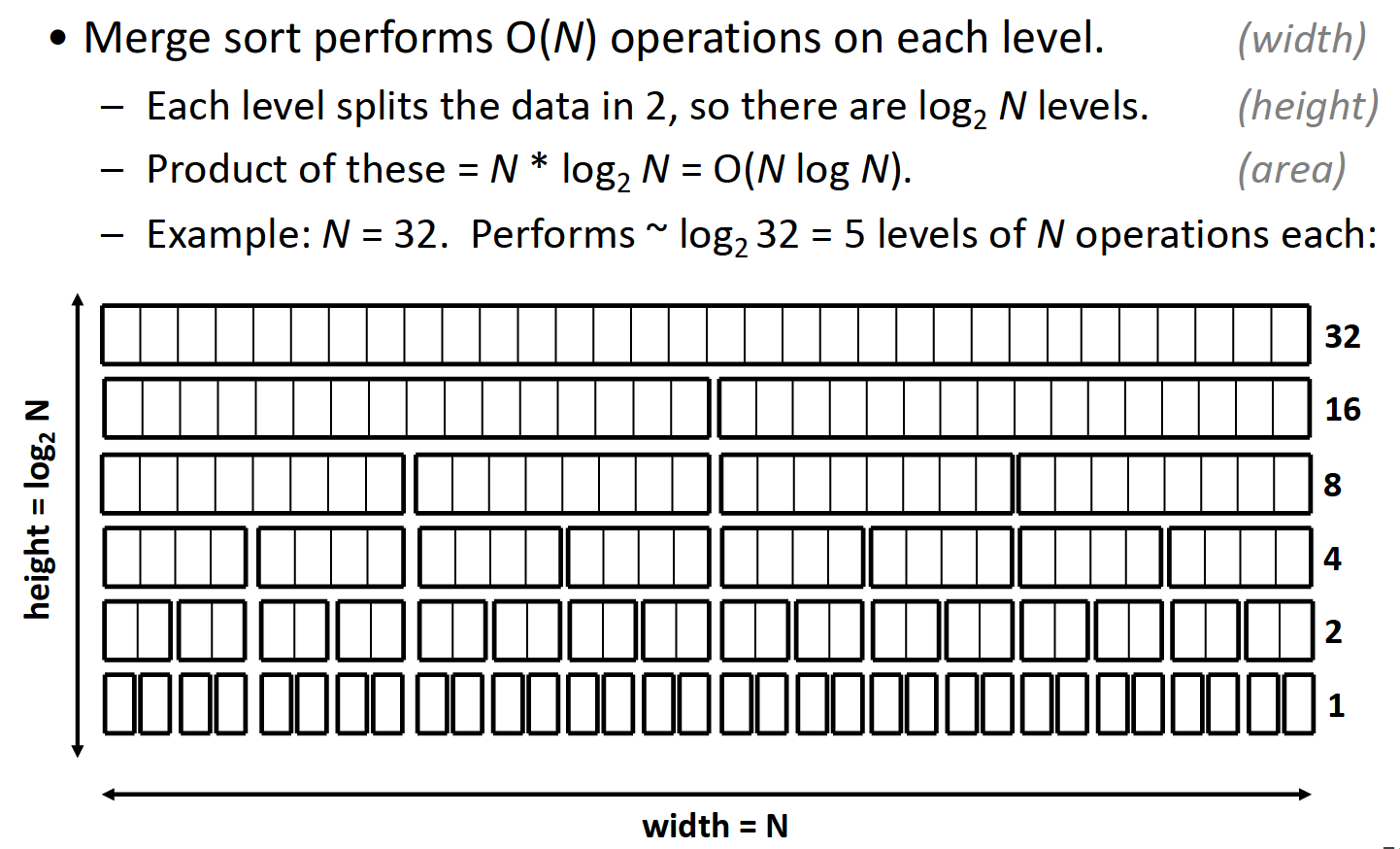
每次merge操作都需要
的时间复杂度,由于每次都将数据分为两块,直到不能继续划分为止,故高度(操作次数)为对数级别,所以最终的时间复杂度为
$$O(nlgn)$$.
quick sort-$$O(nlogn)$$+不稳定
快速排序是使用分治算法的一个典型案例,通过从原数组中选出一个pivot并根据此数值将原数组分为小于pivot和大于pivot的两部分,并把pivot放到合适的位置;再分别从左右两部分中重复此过程…
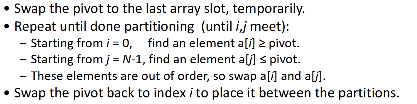
例子:
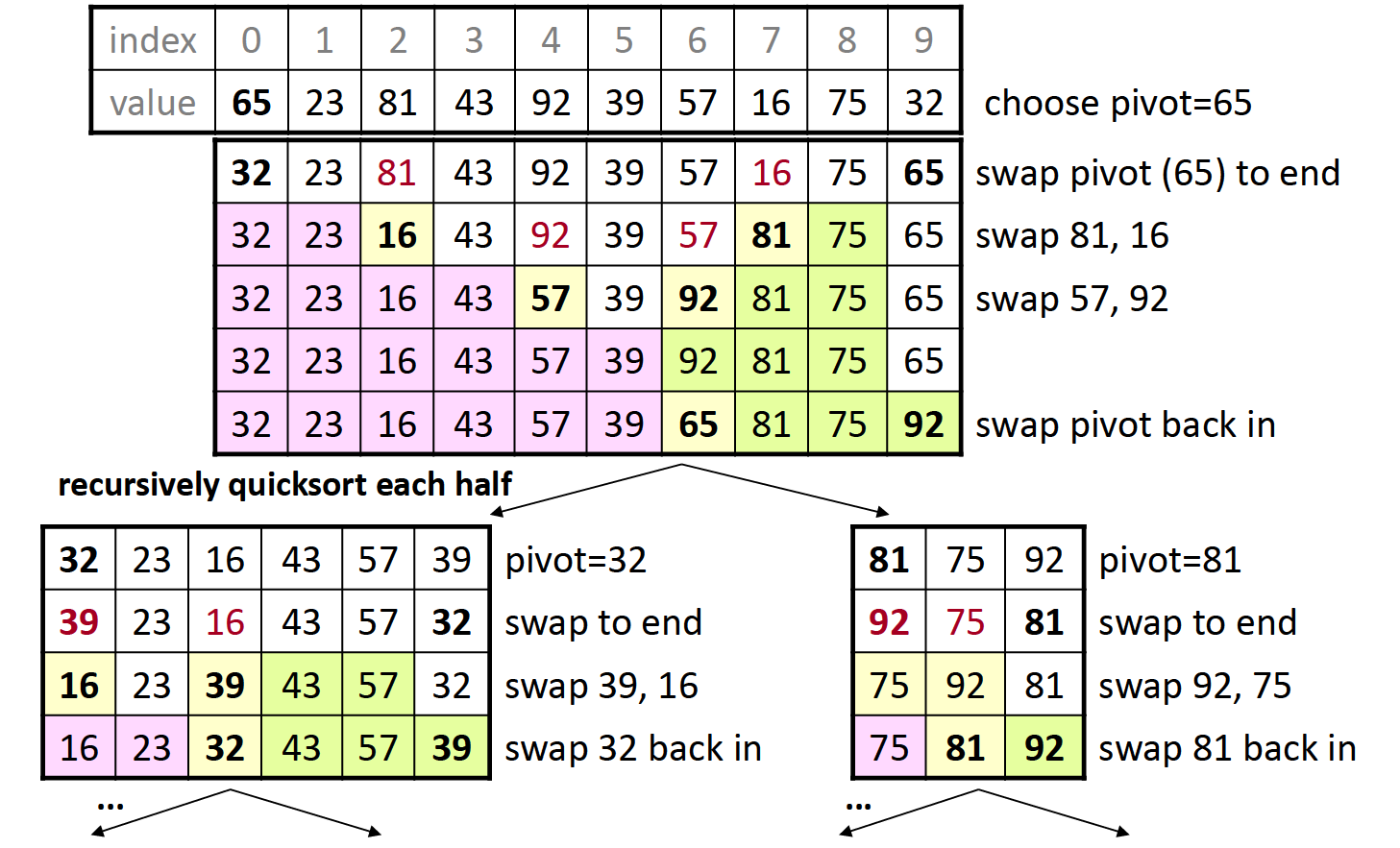
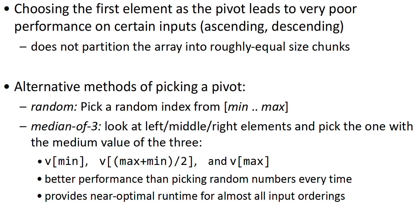
pivot的选择将会直接影响最终的运行效率:
void quickSort(vector<int>& v, int l, int r) {
    // base case:
    if (l >= r) return;

    // 确定分界点
    int i = l - 1, j = r + 1, x = v[l + r >> 1];

    // 调整区间
    while (i < j) {
        do i++; while (v[i] < x);
        do j--; while (v[j] > x);
        if (i < j) swap(v[i], v[j]);
    }

    // 递归处理
    quickSort(v, l, j);
    quickSort(v, j + 1, r);
}
时间复杂度的计算类似于归并排序,也是
$$O(nlgn)$$,且快速排序是一种不稳定的排序算法。
Heap sort-$$O(nlgn)$$+不稳定
堆排序的内容在先前堆的部分提到过,这里不再赘述。
Counting sort-$$O(n+k)$$+稳定
$$k$$为待排序数据的值域大小
常被用作其他排序算法的子程序。这种排序算法不是基于比较的,所以一定是一种稳定的排序算法。算法的基本原理是通过计算得到所有小于某一个数据的元素数目,这样我们便可以得知该数据应当被放到排序数组的哪个位置。所以在实现时,我们需要一个计数数组储存所有数据出现的次数,并把它们的次数从前到后叠加(如果需要降序排列,就从后向前叠加出现次数)。之后便可以利用挨个储存了sumCount的结果的数组(本质上是一个hashTable)得到排序结果了。
// an example
vector<int> v = {9, 4, 10, 8, 2, 4};
void countingSort(vector<int>& v, vector<int>& result) {
    // range of data
    int k = *max_element(v.begin(), v.end()) + 1;
    // the assist array
    vector<int> sumCount(k, 0);
    // First, store the count of elements in the assiat array
    for (int i : v) {
        sumCount[i]++;
    }
    // Second, transfrom the count into sumCount in the assist array
    // if we want to sort the data in descending order, we need to traverse
    // from k-1 to 1
    for (int i = 1; i < k; ++i) {
        sumCount[i] += sumCount[i - 1];
    }
    // Third, use the sumCount to get a sorted array
    for (int i = v.size() - 1; i >= 0; --i) {
        // NOTICE: there should be a minus 1 in the expression
        result[sumCount[v[i]] - 1] = v[i];
        sumCount[v[i]]--;
    }
}
需要注意的是,在第三部分,我们遍历(组成有序数组)的顺序是自后向前,而非自前向后,否则排序算法将不稳定,在之后的基数排序中也能体现出这一点。
时间复杂度因为存在v.size()与k这两个维度,所以最终是
. 如果$$k=O(n)$$,时间复杂度为$$O(n)$$,那么可以考虑使用计数排序算法。
Radix sort-$$O(n\times k)$$+稳定
$$k$$为数字位数
注意到计数排序的使用条件是
$$k=O(n)$$,试想当
$$k=O(n^2)$$时,使用计数排序显然不是一个很好的选择了。但我们可以利用计数排序,或者是任意一种稳定的排序算法,完成基数排序的排序算法。
基数排序的思路其实很简单,就是从低位到高位,针对每一位数字使用稳定的排序算法,分多次对整个序列排序:
void countingSort(vector<int>& v, vector<int>& result, int exp) {
    vector<int> sumCount(10, 0);
    // statistic: number counts
    for (int i : v) {
        sumCount[(i / exp) % 10] += 1;
    }
    // calculate the sumCount
    for (int i = 1; i < 10; ++i) {
        sumCount[i] += sumCount[i - 1];
    }
    // in order, put them into a sorted array
    for (int i = v.size() - 1; i >= 0; --i) {
        result[sumCount[(v[i] / exp) % 10] - 1] = v[i];
        sumCount[(v[i] / exp) % 10]--;
    }
    // change v into result
    v = result;
}

void radixSort(vector<int>& v, vector<int>& result) {
    int max = *max_element(v.begin(), v.end());
    // process each digit from low to high
    for (int exp = 1; max / exp > 0; exp *= 10) {
        countingSort(v, result, exp);
    }
}
时间复杂度简单来说,就是需要对每一位进行排序,而每一次计数排序都是
$$O(n)$$的时间复杂度,所以大致为
$$O(n\times k)$$.
Bucket sort-$$O(n+k)$$+稳定
$$k$$为桶的数量
桶排序主要应用于数据比较均匀的分布在某个范围内时。考虑这样一种情况:数组内的数据全部为小数,那么此时使用计数排序显然不是一个很好的选择,我们可以通过桶排序来完成。我们首先根据桶的总数量计算出要把数据分成的区间数divider,之后计算i/divider可以得到元素需要放入的桶的编号;再将所有元素放入对应的桶之后,对每个桶内元素排序,再把所有元素组合到一起即可。
void bucKetSort(vector<double>& v, vector<double>& result, int bucketNum) {
    double max = *max_element(v.begin(), v.end());
    // how many small ranges we need to divide the data into?
    int divider = ceil((max + 1) / bucketNum);
    vector<double> bucketResult[bucketNum];
    for (auto & i : v) {
        // store the data
        int k = i / divider;
        bucketResult[k].push_back(i);
    }
    // perform sort in each bucket
    for (int i = 0; i < bucketNum; ++i) {
        sort(bucketResult[i].begin(), bucketResult[i].end());
        // concatenate them into the result
        for (auto & j : bucketResult[i]) {
            result.push_back(j);
        }
    }
}
显而易见地,桶排序的时间复杂度为
$$O(n+k)$$,所以如果需要的桶的数量太多,数据分布太广时,这个排序算法的效率会大大下降。
Stanford CS 106X Lecture 29 - Templates, STL, Smart Pointers
Templates
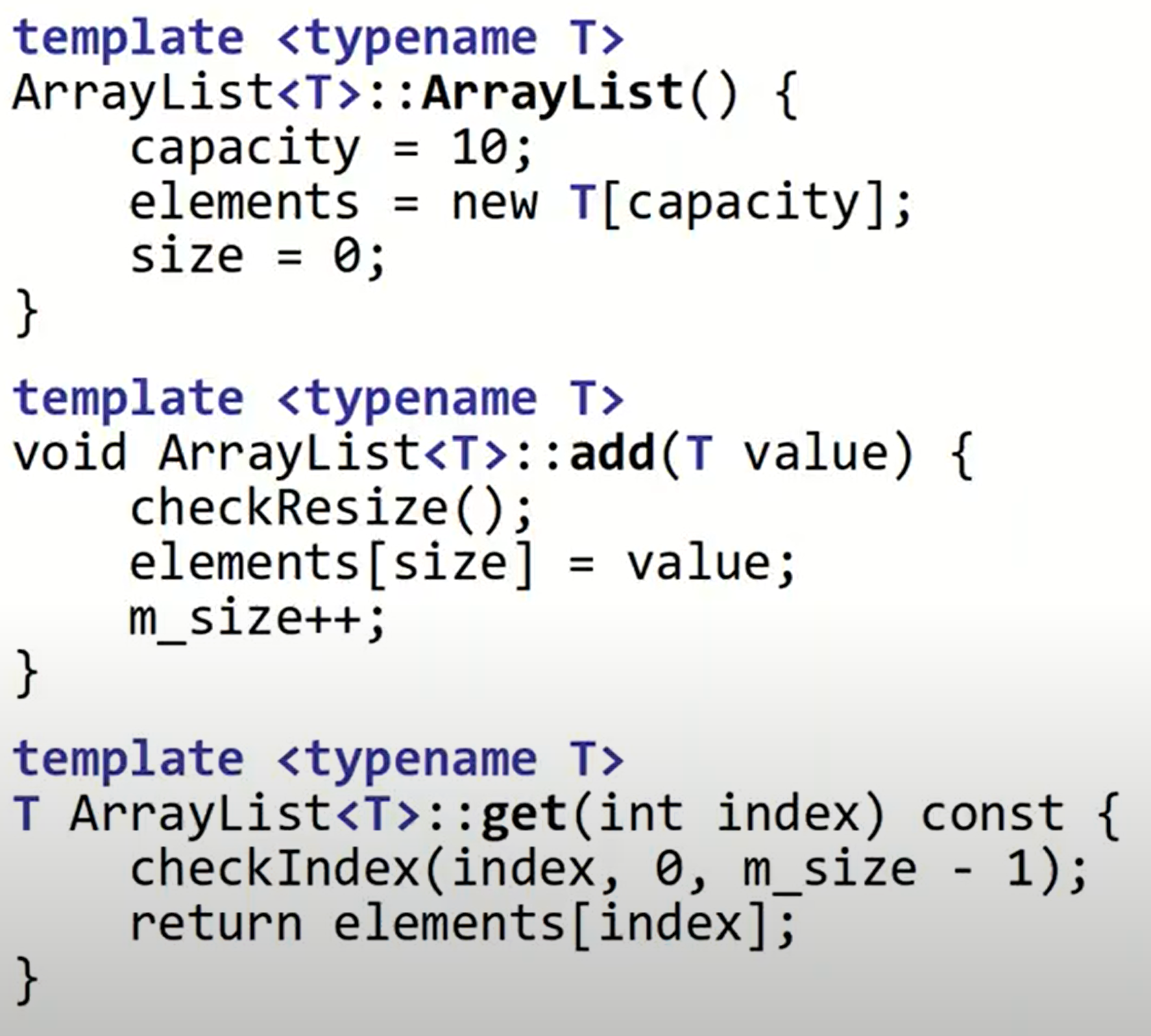
template <typename T>
class ArrayList {
    // statements
}
Smart pointers
smart pointer types:#include<memory>
- unique_ptr (exactly 1 “owner”; best one)
- shared_ptr (multiple “owners”; use sparsingly)
- weak_ptr (use sparingly)
ownership: who is responsible for deleting/freeing the heap-allocated pointer later?
智能指针生命周期结束后,可以自动释放指向的内存,在使用智能指针时,好比是在普通指针外做了一层包裹。
Example:
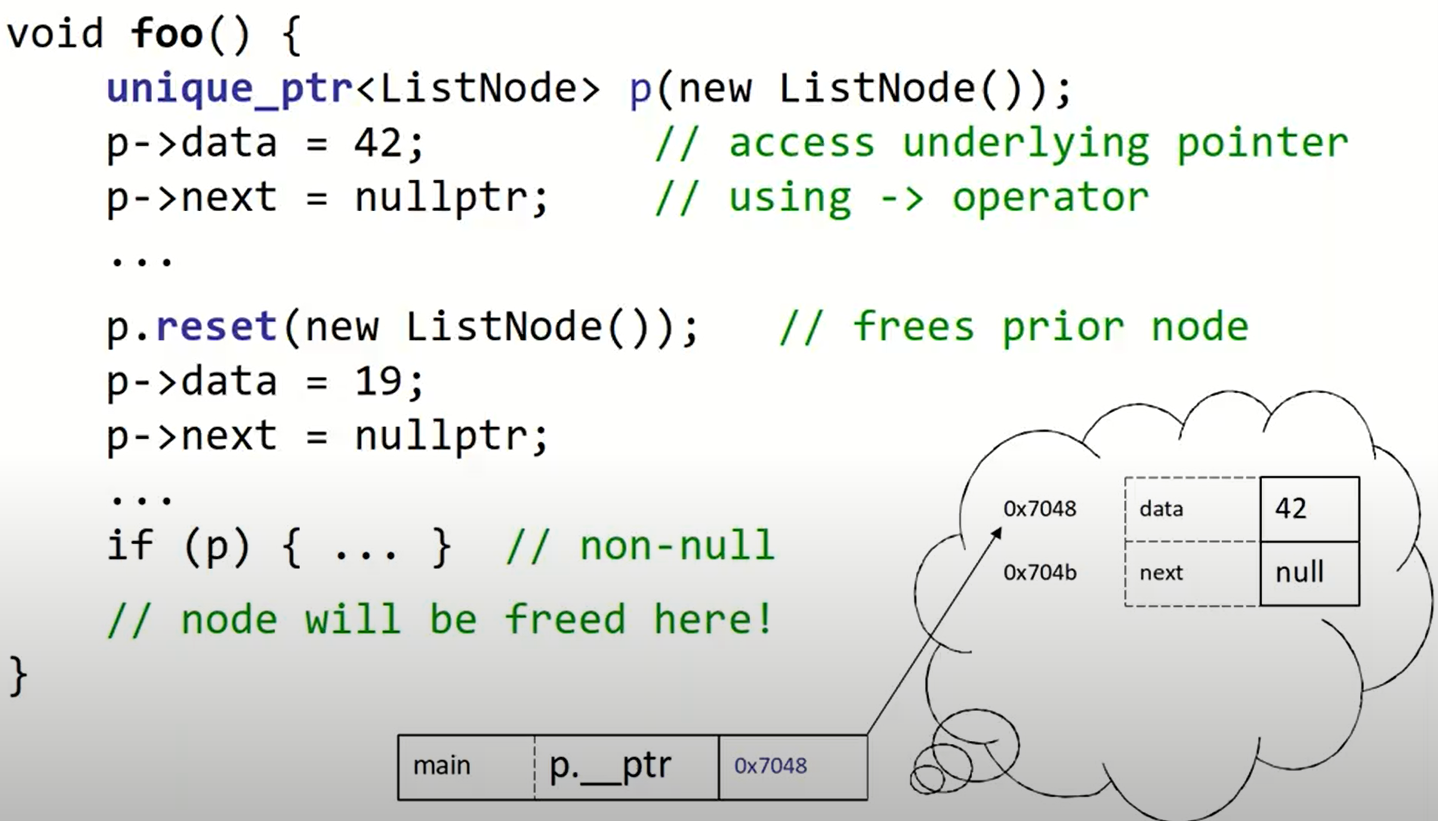
method
unique_ptr<ListNode> p(new ListNode());

// return raw pointer; p still "owns" it
// (and will free it later at end of p's scope)
LIstNode* raw1 = p.get();

// return raw pointer; p stops owning it
// and won't free it any more
ListNode* raw2 = p.release();
unique_ptr as parameter
如果将智能指针直接作为参数,那么程序无法编译!同时,我们要注意也不能使用=对其进行赋值。但是unique_ptr可以作为函数的返回值(move assignment).
二分查找
二叉查找常用于具有单调性性质的题目中,但这不等于说二分查找只能用于具备单调性的题目中。通俗的讲,它的应用条件是我们可以将一个存储分为两个部分1和2,分别满足性质A和不满足性质A,于是二分查找可以帮助我们找到1部分和2部分各自的边界。
二分查找要分为整数二分查找和浮点数二分查找。其中整数查找因为要解决各自的边界问题(中间的分割点有mid, mid + 1),所以更为复杂,存在两种情况,这里我们会用到一个check函数,帮助检查此时的mid满足1部分的性质还是满足2部分的性质,如果我们想要检测2部分的分界(可以理解为区间向后延伸),那么要判断mid是否满足**2(即右侧)**部分具备的性质:
bool check(int x) {/* ... */}

int bsearch_1(int l, int r) {
    while (l < r) {
        // 确定分界点
        int mid = l + r >> 1;
        // 判断mid是否满足(哪种)性质
        // 更新(收缩)判定区间
        // 满足,则当前mid在右半部分分界的右侧,所以可以规定下一次的右边界
        if (check(mid)) r = mid;
        // 不满足,则当前mid在右半部分分界的左侧,所以可以规定下一次的左边界
        else l = mid + 1;
    }
    return l;
}
而如果我们想要检测的是mid是否满足**1(即左侧,可以理解为区间需要向左延申)**的性质:
bool check(int x) {/* ... */}

int bSearch_2(int l, int r) {
    while (l < r) {
        // 确定分界点
        int mid = l + r + 1 >> 1;
        // 更新(收缩)判定区间
        // 满足,则当前mid在左半部分分界的左侧,所以可以规定下一次的左边界
        if (check(mid)) l = mid;
        // 不满足,则当前mid在左半部分分界的右侧,所以可以规定下一次的右边界
        else r = mid - 1;
    }
    return l;
}
两个问题:
- 为什么在对左侧部分寻找性质时,
mid = l + r + 1 >> 1?
即如果
$$mid=\frac{l+r}{2}$$;假设此时
$$l=r-1$$,那么如果左半部分的条件被满足,下一次探寻的范围仍然会是
$$[l, r]$$,程序陷入死循环。而如果
$$mid=\frac{l+r+1}{2}$$就不会出现这个问题。
- 如果二分查找没有找到对应的元素怎么办?
首先,这个问题的定义并不完全正确。之所以找不到元素,并非是因为二分查找算法自身的问题。我们前边提到过,二分查找算法的作用是找到边界,我们可以具化为
$$\ge x$$,但这并不意味着在原本的数据中
$$x$$一定存在。换句话说,如果数据没有找到,问题在于数据集而非二分查找算法,我们最终找到的边界可能是严格
$$\gt x$$的。所以我们可以使用if p[l] != x来判定是否找到了对应的元素。
在实际处理这类问题时,先把mid写作(l + r) / 2。之后根据需要设定的check函数的性质判定需要对l以及r进行的操作,并对mid的值(可能)做+1的变化。
而如果是浮点数二分查找,情况则简单许多。因为我们可以用一条线将数组分为两半,而不用考虑mid,mid + 1的边界问题,所以我们可以统一成一种情况(如果需要做变化改变l, r即可):
bool check(double x) {/* ... */}
double bSearch_3(double l, double r) {
    const double eps = 1e-6;
    while (r - l > eps) {
        double mid = (l + r) / 2;
        if (check(mid)) r = mid;
        else l = mid;
    }
    return l;
}
只是在浮点数二分查找中,我们应当留心eps的设置,一般要比规定的位数再多两个精度。