Basics
- 资源量的计算:两个方面:memory & compute
total_flops公式:$6 \times token\_num \times param\_num$ (对每一个输入的token ,前向要跑过所有的参数,每一个参数都要参与矩阵乘,每个元素都需要经过一次加法和乘法,所以前向需要2TP,反向需要对输出和权重各做一次相同的操作,所以一共需要6TP)
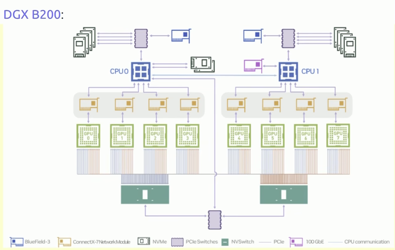
- Scaling Law的建立:用小模型拟合出scale分布曲线(scaling recipe),要求建立比较细致的recipe,包括BS改变的影响等;这是因为一次大规模资源量消耗太大,不可能不断通过大型实验来发现最佳超参;
Tokenization
Encode <-> Decode
可以通过增大词表(vocab size)的方法,来提高压缩比(string -> indices);(因为每个token可以表示的信息可能会变得更多),这会导致:
A. 序列长度更短(对attention友好)
B. sparsity增大,因为有很多embedding可能都不会被学到,这不是好事
BPE_tokenizer
思路:在原始数据上训练tokenizer,得到一个贴合数据的vocabulary;最终让常见的序列可以用一个token来表示,不常见的序列用很多个token来表示;
方法:一开始将每个byte当作一个token,之后不断merge常见的相邻的tokens。
def merge(indices: list[int], pair: tuple[int, int], new_index: int) -> list[int]:
    """Return `indices`, but with all instances of `pair` replaced with `new_index`."""
    new_indices = []
    i = 0
    while i < len(indices):
        if i + 1 < len(indices) and indices[i] == pair[0] and indices[i + 1] == pair[1]:
            new_indices.append(new_index)
            i += 2
        else:
            new_indices.append(indices[i])
            i += 1
    return new_indices


@dataclass(frozen=True)
class BPETokenizerParams:
    """All you need to specify a BPETokenizer."""
    vocab: dict[int, bytes]     # index -> bytes
    merges: dict[tuple[int, int], int]  # index1,index2 -> new_index


def train_bpe(string: str, num_merges: int) -> BPETokenizerParams:
    Start with the list of bytes of string.
    indices = list(map(int, string.encode("utf-8")))
    merges: dict[tuple[int, int], int] = {}  # index1, index2 => merged index
    vocab: dict[int, bytes] = {x: bytes([x]) for x in range(256)}  # index -> bytes
    for i in range(num_merges):
        # Count the number of occurrences of each pair of tokens
        counts = count_adjacent_pairs(indices)
        # Find the most common pair
        pair = max(counts, key=counts.get)
        # Merge that pair
        new_index = 256 + i
        merges[pair] = new_index
        vocab[new_index] = vocab[pair[0]] + vocab[pair[1]]
        indices = merge(indices, pair, new_index)
    compression_ratio = get_compression_ratio(string, indices)
    return BPETokenizerParams(vocab=vocab, merges=merges)

def count_adjacent_pairs(indices: list[int]) -> dict[tuple[int, int], int]:
    """Return a dictionary mapping each adjacent pair of tokens in `indices` to the number of times it occurs."""
    counts = defaultdict(int)
    for index1, index2 in zip(indices, indices[1:]):
        counts[(index1, index2)] += 1
    return counts


class BPETokenizer(Tokenizer):
    """BPE tokenizer given a set of merges and a vocabulary."""
    def __init__(self, params: BPETokenizerParams):
        self.params = params
    def encode(self, string: str) -> list[int]:
        indices = list(map(int, string.encode("utf-8")))
        # Note: this is a very slow implementation
        for pair, new_index in self.params.merges.items():
            indices = merge(indices, pair, new_index)
        return indices
    def decode(self, indices: list[int]) -> str:
        bytes_list = list(map(self.params.vocab.get, indices))
        string = b"".join(bytes_list).decode("utf-8")
        return string
Resource Accounting
Einops
- motivation: 因为使用普通的pytorch矩阵行列变换操作很容易出错,einops方便我们对dimension进行操作;
x = torch.ones(3, 4)
y = torch.ones(4, 3)

# --- sum ---
z = x @ y
# 等价于
z = einsum(x, y, "seq1 hidden, hidden seq2 -> seq1 seq2")

z = x @ y.transpose(-2, -1)
# 等价于 (或者手动将...写成'batch')
z = einsum(x, y, "... seq1 hidden, ... seq2 hidden -> ... seq1 seq2")

# --- reduce ---
y = x.sum(dim=-1)
# 等价于
y = reduce(x, "...hidden -> ...", "sum")

# --- rearrange ---
# (3, 8) -> (3, 2, 4),或者反过来也可以
x = rearrange(x, "...(heads hidden1) -> ... heads hidden1", heads=2)
Flops of matmul operation
x: (B, D), w: (D, K) 每个位置包含一次加法和乘法,故flops为$2*BDK$
- B是点的数量
- (DK)是参数的数量
那么对于一次前向的矩阵乘法,flops就是$2\*tokens\*params$,也是前边整体flops计算公式的由来。
MFU
MFU: Model FlOPS Utilization = actual flop_per_second / promised flop_per_second
promised flop per second: 可以在设备指标中找到
一般大于等于0.5的MFU就算是很好了.
arithmetic intensity
两个组件:计算单元& memory,所以计算耗时取决于两个因素:
- Accelerator speed (FLOP/s)
- memory bandwith (bytes/s)
衡量程序是compute boundh还是memory bound有两种方法:
首先可以比较communication time和compute time:
- communication time: bytes / h100_bytes_per_second
- compute time: flops / h100_flop_per_second
我们假设通信和计算可以overlap,那么:
- memory bound: communication time > compute time
- compute bound: compute time > communication time
另一种等价的衡量方式:
- Accelarator intensity: h100_flop_per_second / h100_bytes_per_second
- Arithmetic intensity: flops / bytes
那么:
- memory bound: Accelerator intensity > arithmetic intensity
- compute bound: Arithmetic intensity > accelerator intensity
example: matmul
bytes: 2nn+2nn+2nn
Flops: nn(2n-1)
只要matrix足够大,就是一个compute bound的操作。
为什么推理过程是memory bound的?因为推理大多做的是matrix-vector multiplication.
    n = 1024
    x = torch.ones(n, dtype=torch.bfloat16, device=cuda_if_available())
    w = torch.ones(n, n, dtype=torch.bfloat16, device=cuda_if_available())
    y = x @ w
    bytes = (2 * n) + (2 * n * n) + (2 * n)  # Read x, read w, write y
    flops = n * (2 * n - 1)  # n dot-products
    arithmetic_intensity = flops / bytes  # ~1
H100_accelerator_intensity » arithmetic intensity
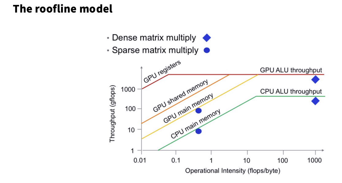
roofline plots
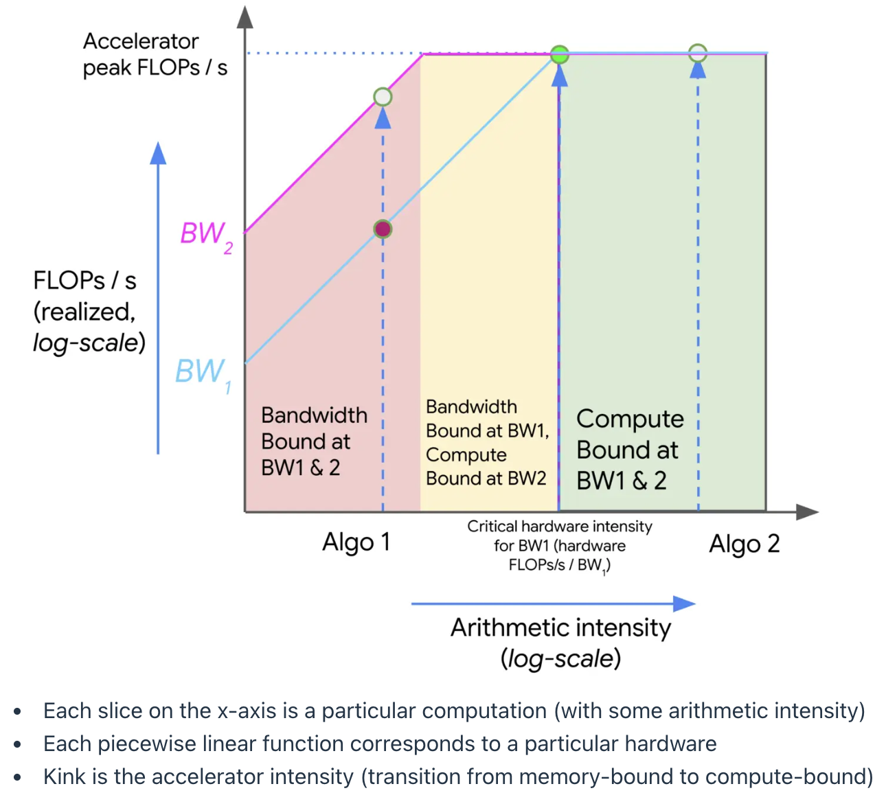
在前期,如果搬运每个byte所对应的计算操作很少,那么显然大部分资源都被浪费在memory上,而非计算单元内。
Architecture
Layernorm
Pre-vs-post norm
将$x_i$->$x_{i+1}$的通路称为residual stream,目前主流的方法是右侧的pre-norm,即在mha和FFN之前做layer norm. 因为不在residual stream上,所以也被称为non-residual norm.
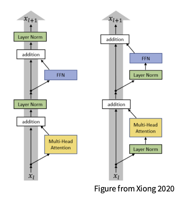
优势:
- 即使不经过warmup,也可以有相比post-norm更好的稳定性,更少的gradient spike现象。
现在还有一种方法是在计算之后也加上layernorm:
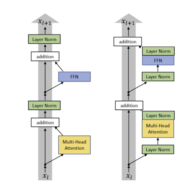
也被叫做double norm.
Layernorm vs. RMSNorm
观察这两者的公式区别:
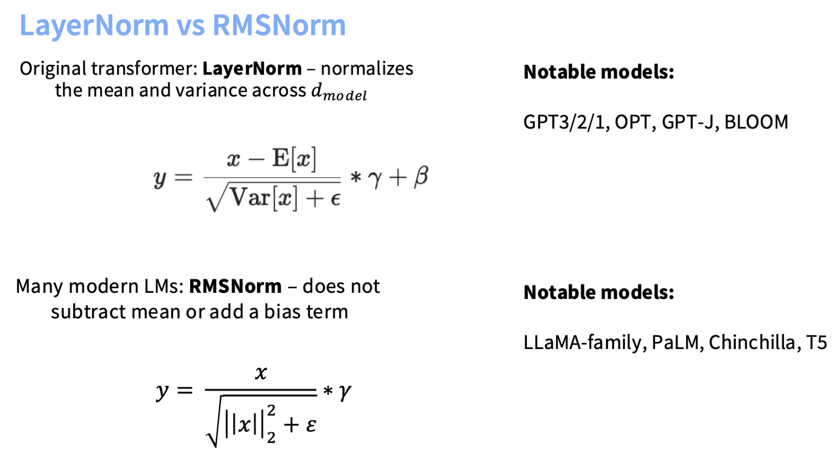
RMSNorm相比layernorm,有着更少的操作(不需要计算mean)和更少的参数(没后bias term),事实上这两个diff对性能的提升至关重要:
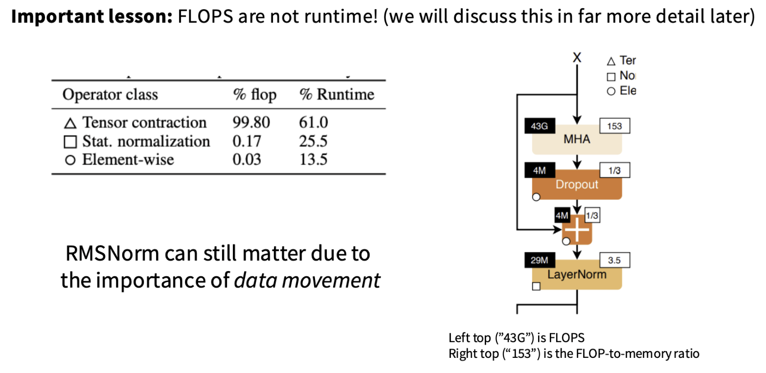
可以看到虽然normalization和element-wise的bias term计算的flop很少,但是占用的时间却很长。
在现代的LLM transformer架构中,bias term也经常是没有的.
Activations
一个architecture设计的经验之谈:gating往往很有帮助;其实就是一个矩阵乘法。
比如在activation的设计中,从relu到**GLU的演化就是多了一个gate function:
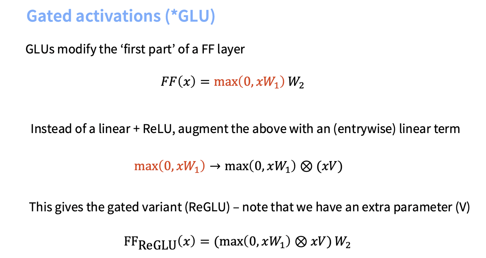
各种GLU的不同就在于新增加的参数矩阵V的选择的不同,对于目前最通用的SwiGLU,选择的是一个$sigmoid(x)$:
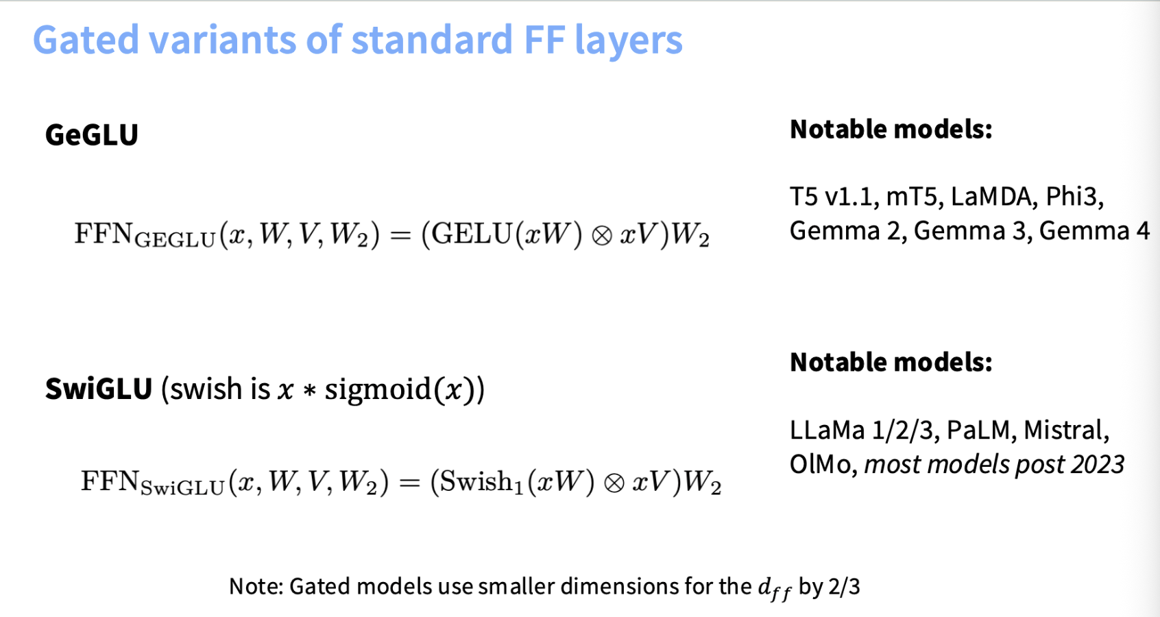
这里的一个小细节是为了让总参数量和之前一样(因为增加了一个新的权重矩阵v),对dim需要进行缩减。
Serial vs. Parallel layers
GPTJ ,PaLM, GPT-NeoX等模型提出了将原本序列化运算的transformer结构改造成parallel的:
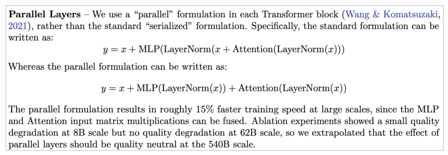
但目前不常用。
位置编码
参考资料:
- https://kazemnejad.com/blog/transformer_architecture_positional_encoding/
- https://zhuanlan.zhihu.com/p/721032991
- https://spaces.ac.cn/archives/8231
- https://zhuanlan.zhihu.com/p/642884818
- https://mp.weixin.qq.com/s/-1xVXjoM0imXMC7DKqo-Gw
- https://kexue.fm/archives/8265/comment-page-2
- https://mp.weixin.qq.com/s?__biz=MzA3MTgwODE1Ng==&mid=2247484826&idx=1&sn=8935f0bcb2e09f438cbf3ae63825d671&chksm=9f26a069a851297f568ba7cd111082e603108716928b8444a253457233f24d09d3a18447d6b9&cur_album_id=3199751010206973953&scene=189#wechat_redirect
- 为什么要有位置编码?
因为attention结构本身无法捕捉token顺序。
位置编码有以下几个要求:
- 能够表示一个token在序列中的绝对位置;
- 能够用绝对位置表示token间的相对位置;
- 具有外推性,即可以表示模型在训练过程中没有见过的长度;
Sinusoidal位置编码
正余弦位置编码的思路来自于位置本身的二进制表示,提供了一种有界又连续的编码方法:
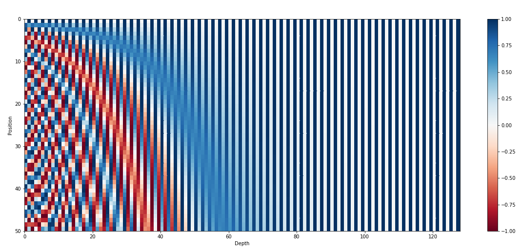
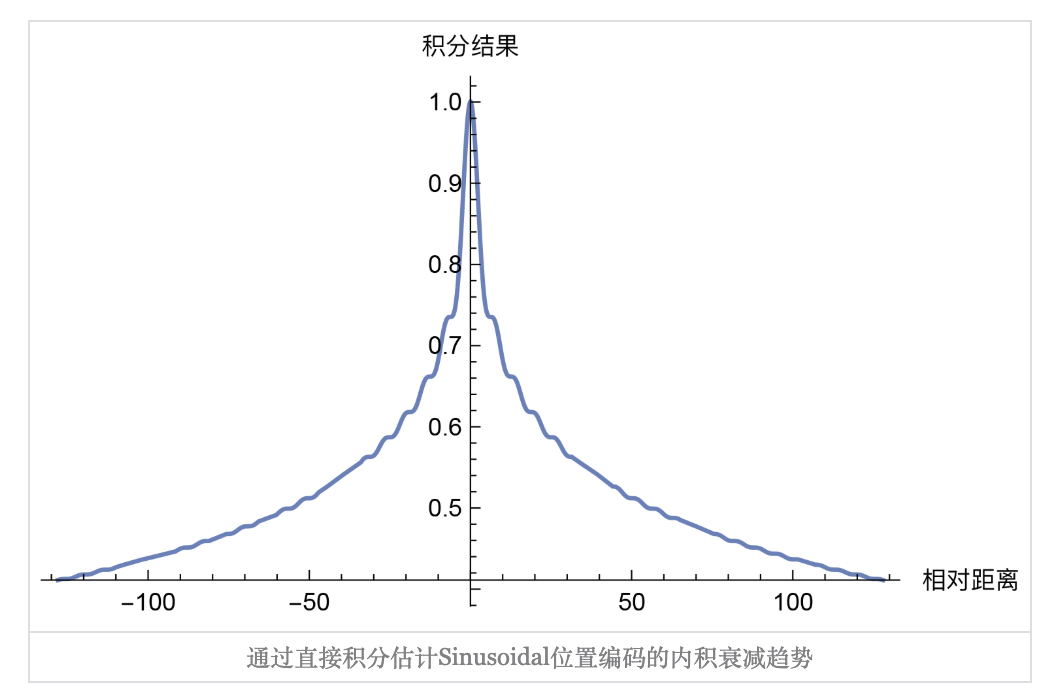
- 为什么$\omega_k = \frac{1}{10000^{2k / d}}$?
为了满足设想:相关距离越远的embedding,相关性应该越小;也即远程衰减性:
- 绝对位置编码如何表达相对位置信息?
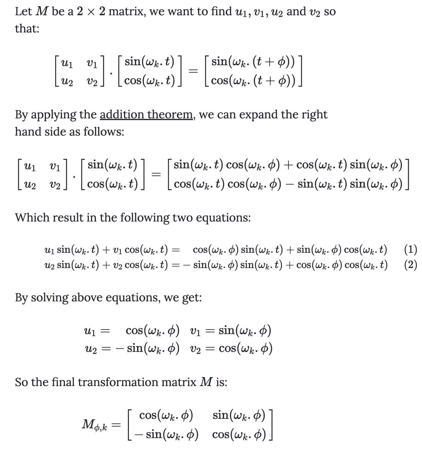
ROPE
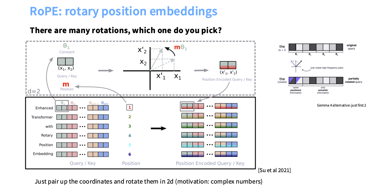
对于二维向量:
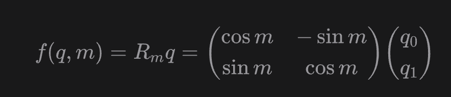
即在向量上乘上一个旋转矩阵,同样地对于多偶数维向量,可以将其两两分组(注意这里的$\theta$对每个d的值是不同的),我们接下来会证明为什么这个形式是可以表达相对位置信息的;
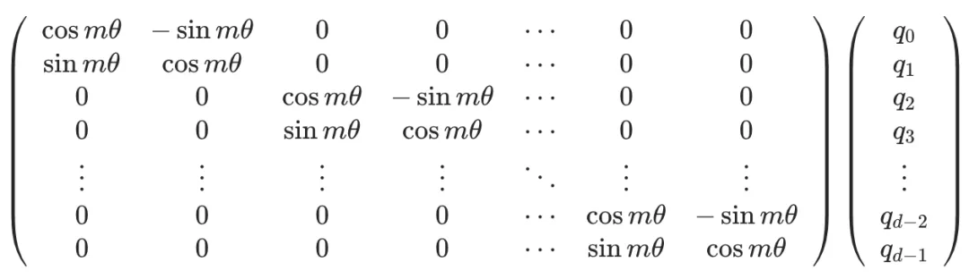
上式中的旋转矩阵十分稀疏,为了节省算力,可以以下面的方式等效实现:
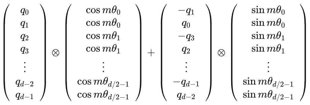
上述公式里$\theta$的取值可以复用先前正余弦位置编码的方法,同样带来一定的远程衰减性。
- ROPE是如何用绝对位置编码表示相对位置信息的?
我们考察二维下的ROPE,注意到其相当于在embedding上乘了一个旋转矩阵,设旋转矩阵为$R$,那我们尝试证明:
$$注意到旋转矩阵的性质:
- $$R_a^T=R_{-a}$$
- $$R_aR_b=R_{a+b}$$
则:
$$那么对于高维向量,由于内积具有线性性质,即$
- ROPE为何具有外推性?
本质上是因为旋转矩阵的存在,让位置编码具备了周期性和远程衰减性,这两个性质允许我们做类似线性插值(将推理时没有见过的旋转角度恢复到训练时见过的角度范围内),以及后续的优化高频信息的NTK插值等方法,通过缩小旋转弧度$m\theta_i$达到长度扩展的目的,具体参见参考文章的最后一篇内容。
Hyperparameters
- Feedforward-model dimension ratio
对transformer中的FFN层的一般形式:
$$FFN(x)=max(0,xW_1+b_1)W_2+b_2$$其中,$d_{ff}$表示中间层的输出维度,$d_{model}$为transformer层的输出维度。
一般都有$d_{ff}=4d_{model}$或者$d_{ff}=2.66d_{model}$.
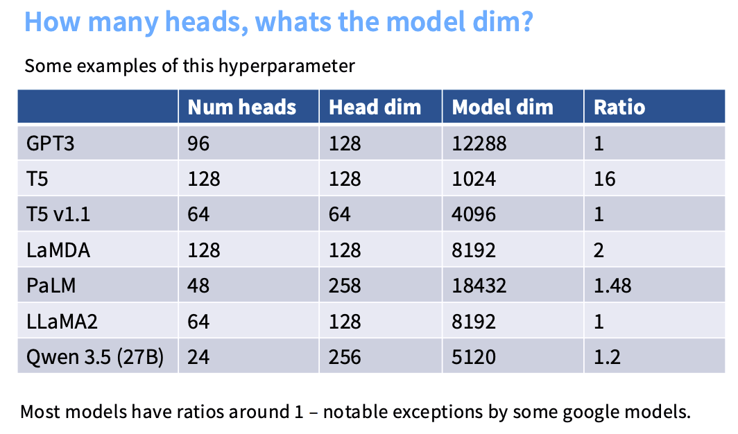
- Head_dim * num_heads to model-dim ratio
基本会保持model dim是head dim * num_heads的整数倍,大部分是1:
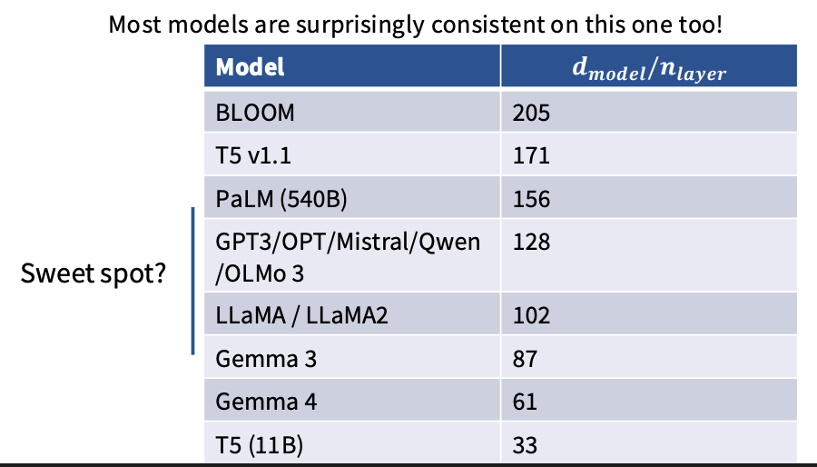
- Aspect ratios
表征模型的宽度和深度的比值,主要考量在于如果模型过深,可能需要通过PP来做并行切分,对性能有影响,对效果的影响则并非主要因素。大部分模型的d_model / n_layer都在100左右:
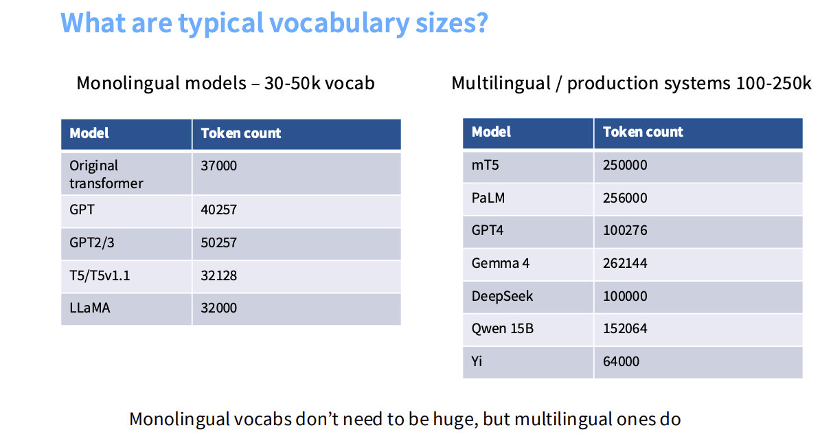
- vocab sizes
- Dropout and other regularization
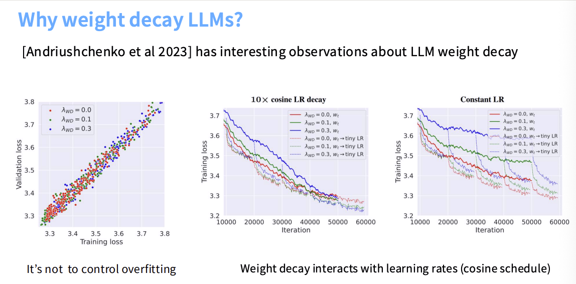
在预训练时,因为有很多数据,同时SGD只在语料库上跑一遍,所以想要overfit不太容易,所以有weight decay和dropout的必要吗?大部分现代LLM仍然会做dropout & weight decay,但其目的并非为了防止overfitting,而是在动态优化上(比如和lr decay结合给模型带来的收敛加速)上有优势:
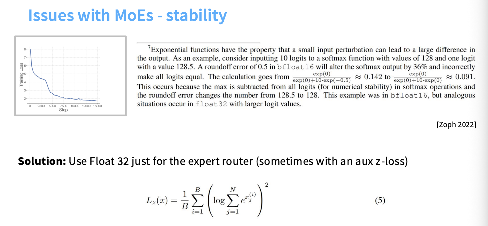
stability issue
Softmax
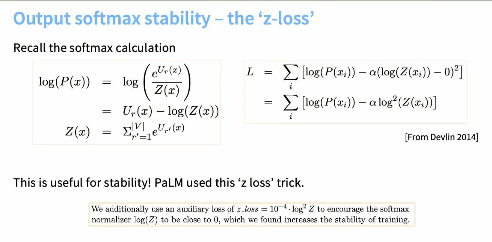
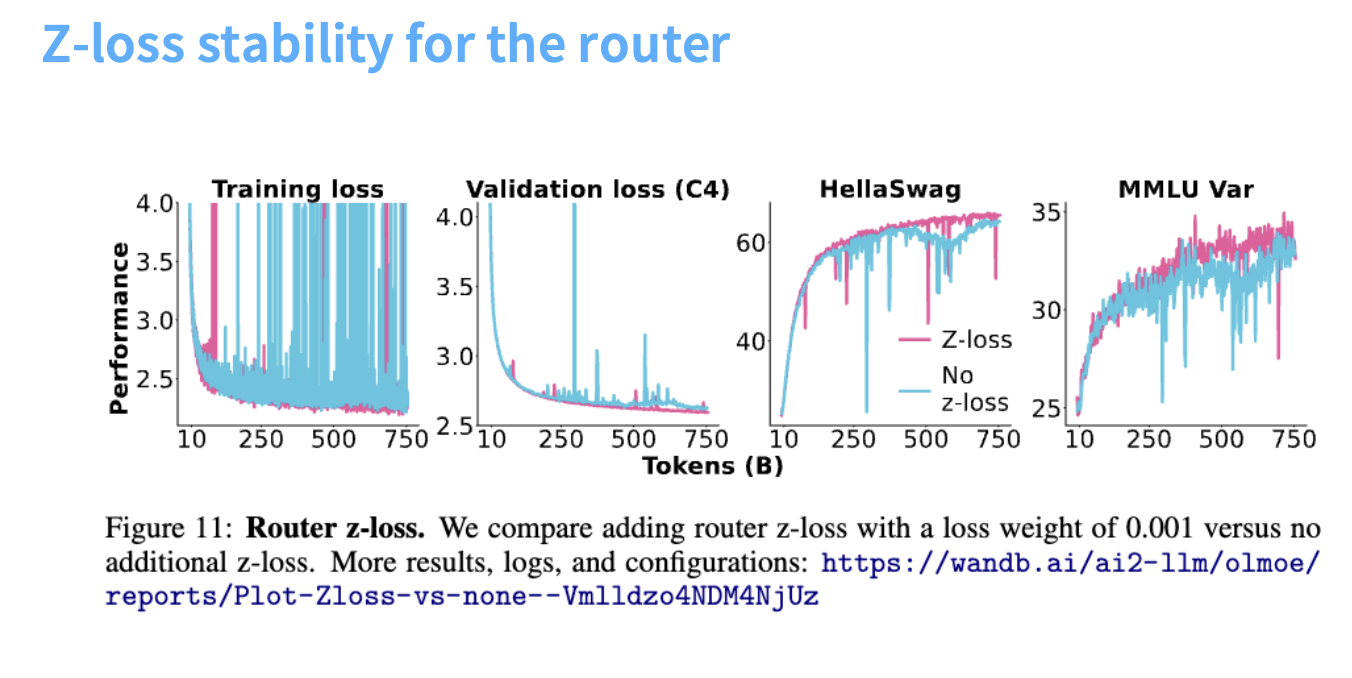
- Output softmax stability - z-loss
通过增加一个z-loss的正则化项,因为我们在尝试最小化loss,所以这样可以让Z(X)贴近1,从而达到稳定Z(x)的目的.
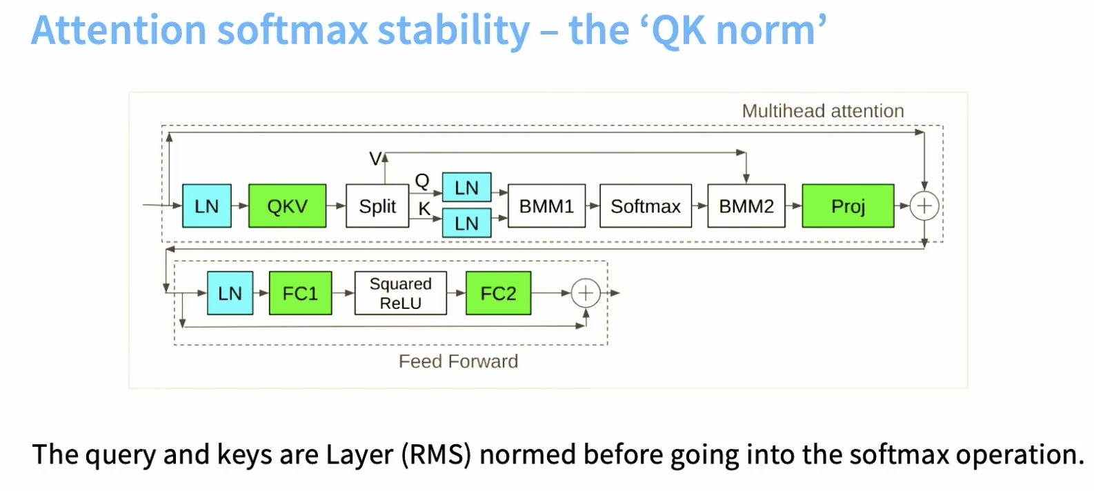
- Attention softmax stability - QK norm
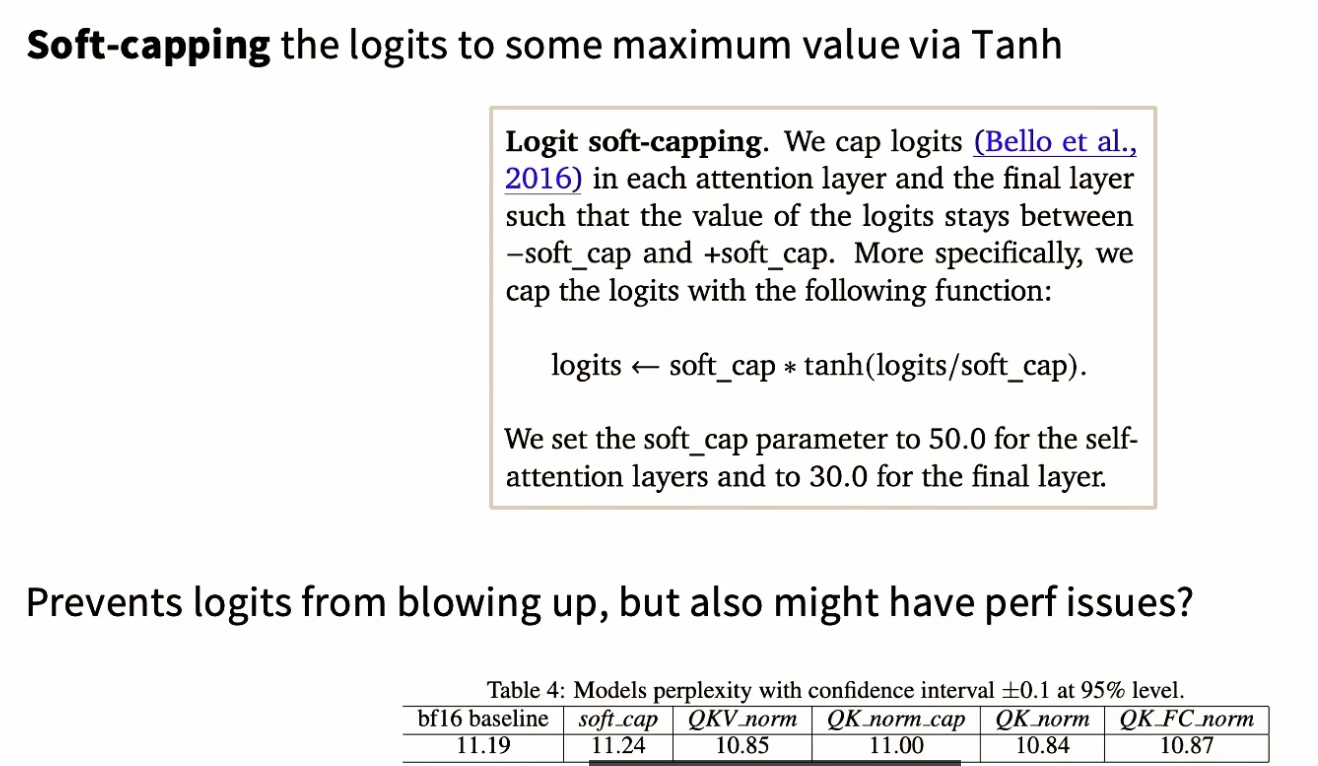
Logit soft-capping
Attention heads
除了以下几个例外,大部分模型对attention heads都不会有改动:
- GQA/MQA (Reduce attention head cost)
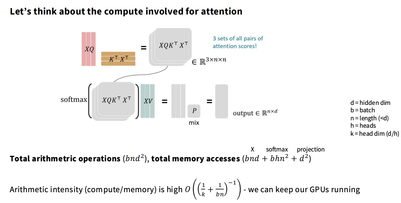
以上图为例,计算操作的结果源于n<d,所以在projection和attention两个矩阵乘法中,前者占了上风,如果此时的场景换成长文本,即n » d,那么结果应当为$O(bn^2d)$。
上述场景发生在训练以及推理的prefill阶段中,但是在decode阶段,假设此时也有N个query token逐次进来:
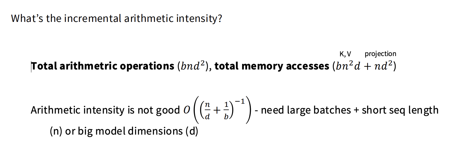
- arithmetic operations: 仍然是proj占据上风,n次的(b*1*d) @ (d*d),所以仍然是O(bnd^2);
- total memory access: n次的(b*n*d)还有n次的对proj矩阵(d*d)的访问;
这里忽略了softmax的访存,因为比kv读取少一个n的量级,同时因为推理阶段没有backward,所以可以不把softmaxx结果写回HBM.
在decode阶段的计算强度很低,最好需要大batch+短序列,或者模型dim很大,对于小模型不太友好,
MQA正是为了解决上述痛点。
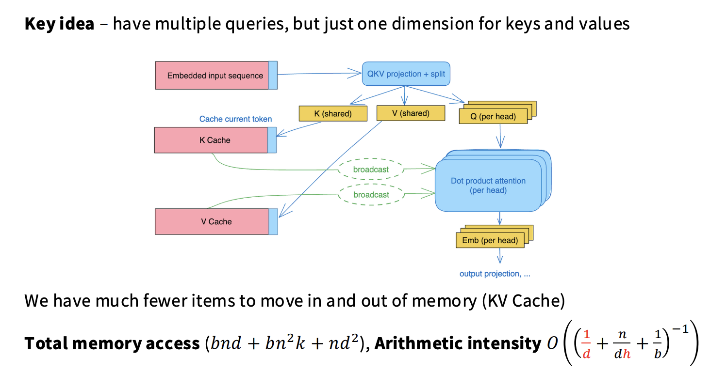
这里多出的第一项是对Q的读取,先前MHA没有列出来,是因为当时有$bn^2d$的存在。
但是MQA的问题在于因为head太少,确实会丢失expressiveness (key-query ratio),所以变成了GQA:
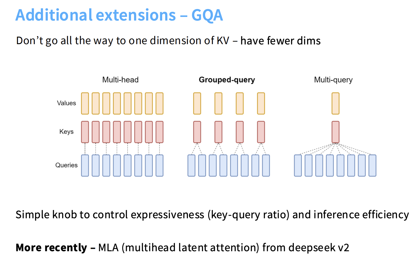
在训练时repeat
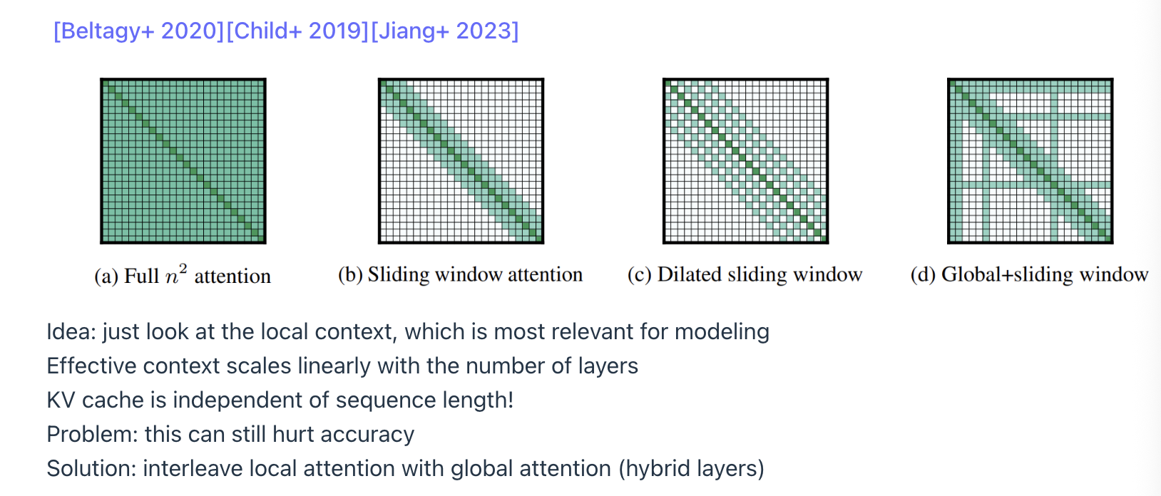
- Sparse / sliding window attention
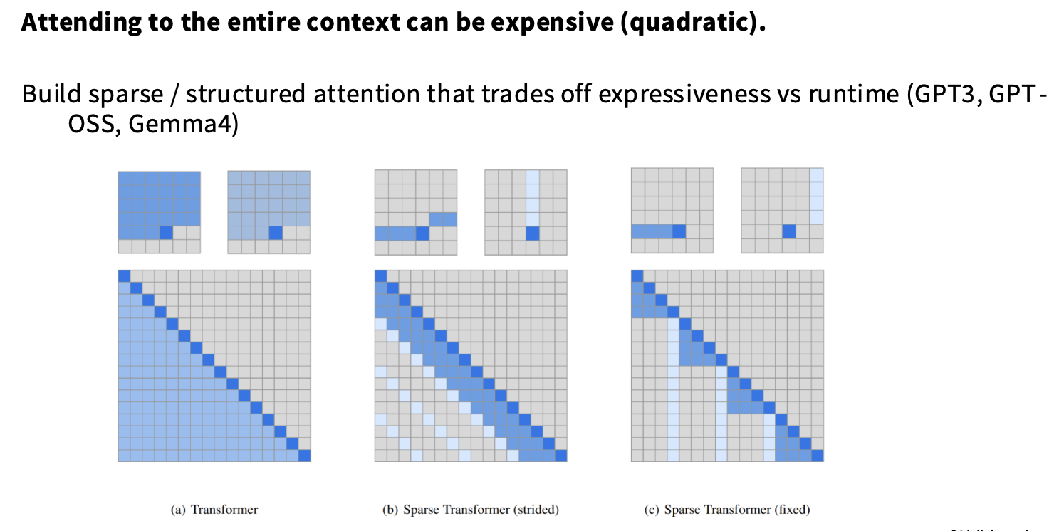
现在比较流行的做法是在full attention和sparse attention之间交替。
Long-range info via NoPE, short-range info via RoPE + SWA.
Attention Alternatives and MOE
Linear attention
Linear attention的核心思路是思考:如何将(QK^T)V变成Q(K^TV),其好处在于将O(N^2d_k+N^2d_v)的计算复杂度降低到O(2N*d_v*d_k).
核心问题在于softmax不是一个满足结合律的操作,即做上述交换之后,效果不等价,所以当前linear attention会使用elu/silu等其他函数,具体细节可以参考网上的其他文章。
linear attention的优劣明显:
- 优势:降低计算复杂度,适合推理,原因:可以表示成类似RNN的形式:

- 为什么可以表示成这种形式?
$\phi(QK^T)V$ -> $Q\phi(K^TV)$,令$S=K^TV$,$S$的shape为$(d\times d)$,注意到$K=[K_0, K_1,...,K_n]$,$V=[V_0, V_1, ..., V_n]^T$,则$S=\sum^n_{i=0}K_iV_i$,那么显然有$S_{i+1}=S_i+K_iV_i$,在训练和推理时都适用。
- 这种形式有什么好处?
可以大幅降低KV cache size,提升推理速度(因为read/write减少),相比于之前要保存每一轮推理后更新的KV矩阵,现在只需要保存S矩阵即可,而S矩阵是一个$d\times d$的矩阵。
因为推理时的token是逐个喂进来的,所以这种串行形式适合推理。
- 劣势:不适合训练,因为无法并行:由于casual mask的存在,导致对每个Q token,不能使用一致的K^TV矩阵,必须按照上边展示的那种kv逐次递增的方法来做。
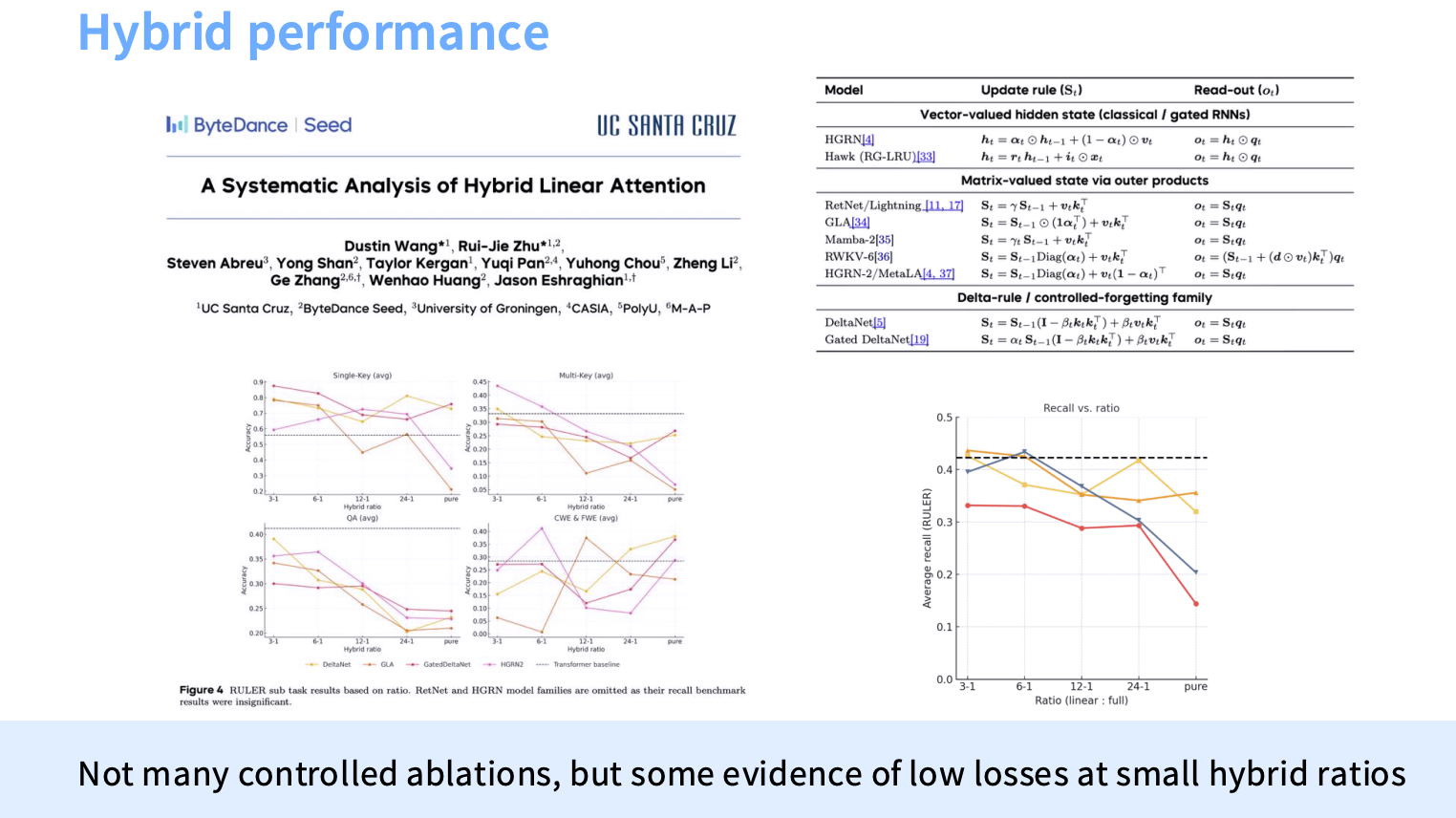
但是这种方案会有效果问题,所以在实际使用中,例如Minimax M1,使用了hybrid attention的方案,即interleave full attention和linear attention,根据研究表明,两者比值并非线性关系,但有一些证据表明在较低的linear/ratio比值下,模型效果较好。
Lightening attention
在linear attention的基础上,产生了lightening attention。
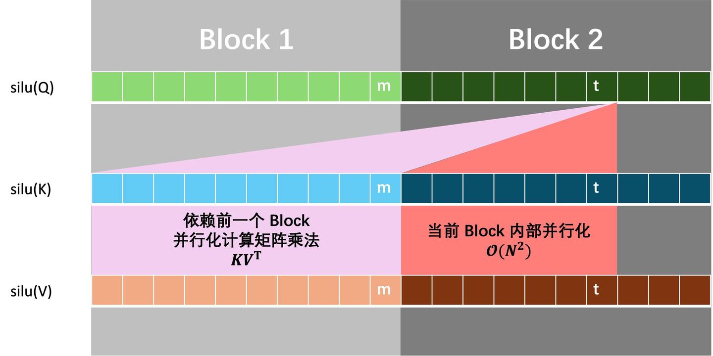
其在linear attention的基础之上,融合了flash attention的想法,即将完整的token序列切成多个block,分段计算attention。
对于每一个需要依赖先前pos 0-m (属于block1)的pos m+t (属于block2),从0-m段的attention计算时,缓存中间结果K^TV,并使用linear attention递推到第m位,这样做的好处在于对于长序列场景,前边的所有位置都降低到线性时间复杂度;这在方案中被称为inter block;而对于block2内部的[m+1, m+t)则仍然采用parallel形式的QK^T做计算,充分利用tensor core加速,这在方案中被称为intra block。
此外,采用了类似FA的cache策略,即做inter_ret + intra_ret的cumsum时,在SRAM中进行等。
Future Reading: https://www.zhihu.com/question/9740764576
Mamba-2
可以理解成在linear attention上加了一个gating:
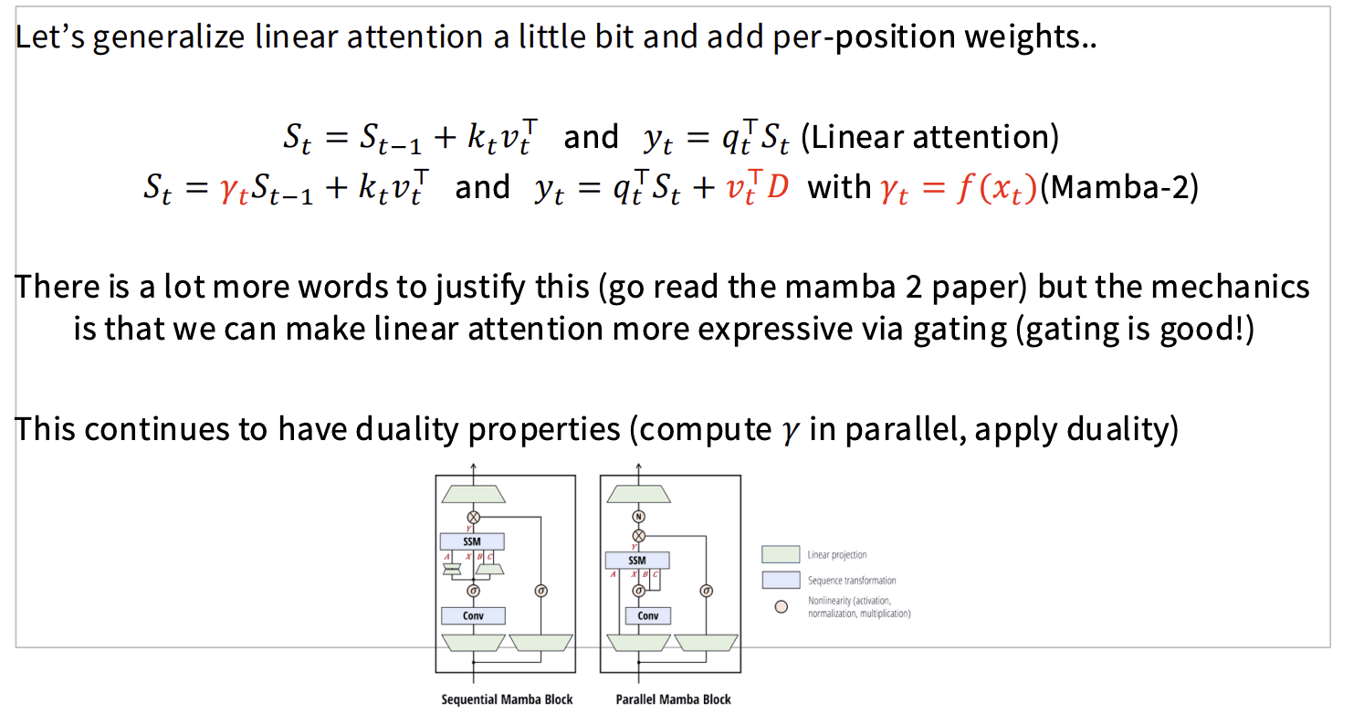
作用是动态遗忘或保留历史信息,从而更有表达力。
Nemotron 3使用了该方案.
Gated delta net
在mamba-2的基础上衍生而来,通过一个投影矩阵$k_tk^T_t$消除历史信息的影响:
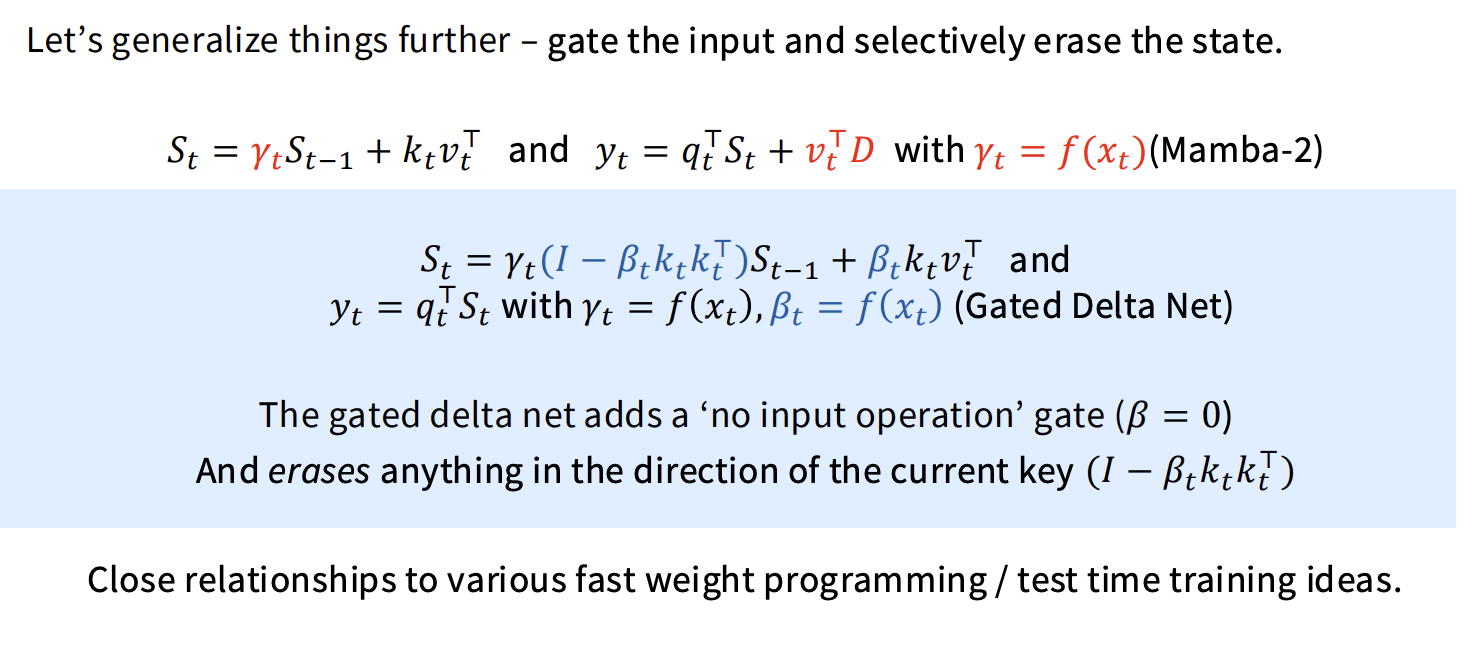
至于为什么该矩阵是一个project out的作用,可以参考投影矩阵对应的介绍资料,这里不再赘述。
Qwen 3.5 / Qwen Next使用了该方案.
Sparse adaptation
典型例子:DSA:
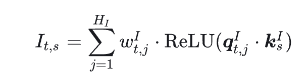
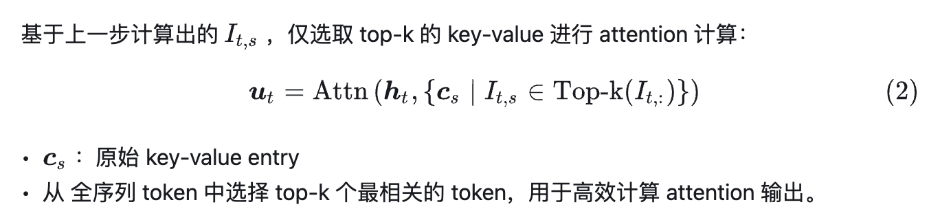
虽然计算复杂度仍然是平方级别的,但因为有indexer的存在,导致复杂度的常数项小了很多,整体复杂度降低。
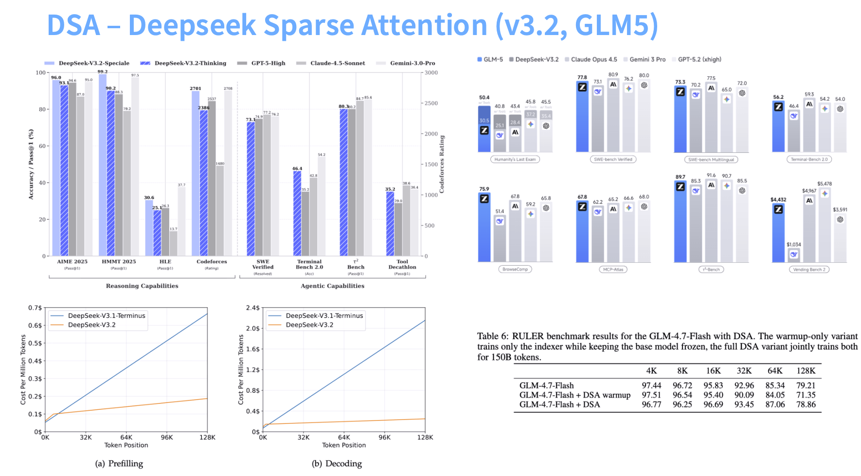
参考资料:https://zhuanlan.zhihu.com/p/1959636888123049941
MOE
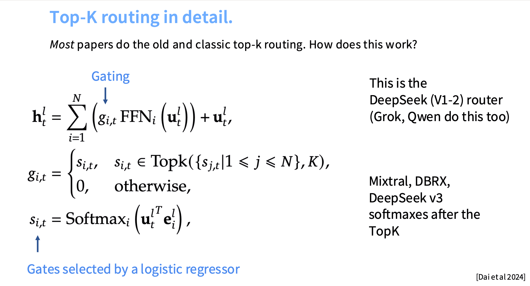
老式的MOE做法是:
先计算出所有expert的routing logits,过一层softmax,把softmax的输出结果作为topk的score,再将topk的结果作为gating function,但这种方法会导致最后topk的概率和不为1,所以在之后的模型结构中,大部分改为在topk之后,只在selected experts上做softmax。
- Shared experts
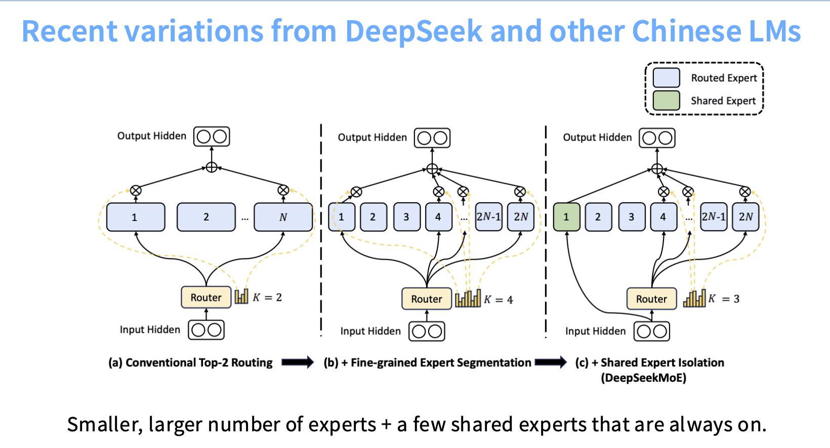
对于shared expert能否提高效果,说法不一,但是将expert切的更细,即fine-grained expert。
Train MOEs
虽然sparsity带来了训练阶段的高效性,但因为gating+topk操作不可微分,这给通过正常的梯度下降更新带来了困难;所以训练MOE模型需要一些trick。
- 使用强化学习更新门控策略: 可以做,但是太复杂,不常用;
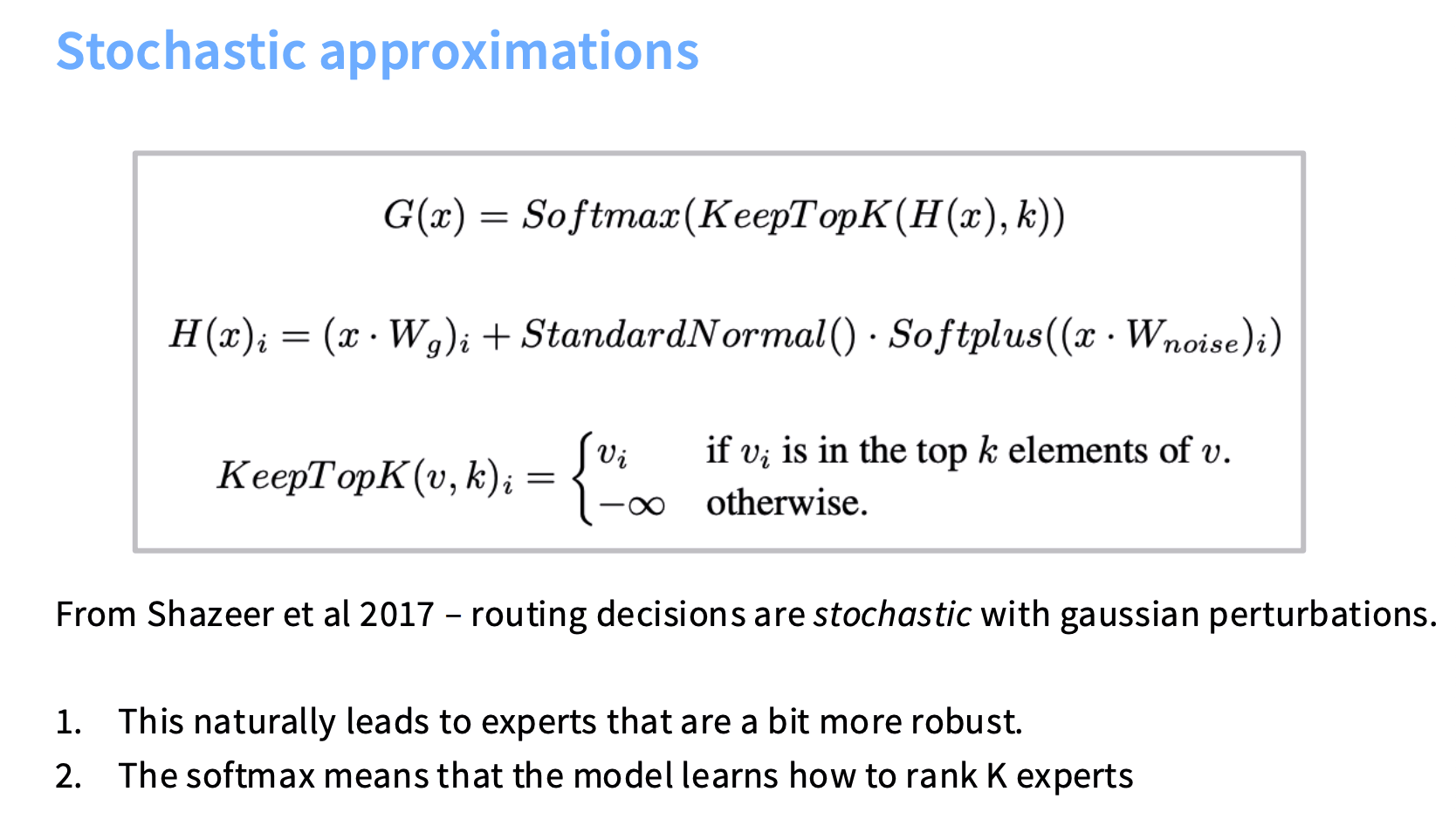
- 增加随机扰动项(
stochastic perturbations):
- 启发式平衡loss(
Heuristic balancing losses)
在原版的total loss基础上,增加一个辅助loss(auxiliary loss),目的:如果一个expert获得了过多的token,那么会压制接下来token选择该expert的概率。由两部分构成:
$f_i$表示被路由到$E_i$的比例,$P_i$表示被路由到$E_i$的平均概率,那么:
$$loss=\alpha N \sum_{i=1}^N f_i P_i$$- 需要有f,因为被路由的概率只是一个软性的指标,不代表最后dispatch的结果;
- 需要有p,因为f不可微分,需要p作为可微入口,将梯度回传router;
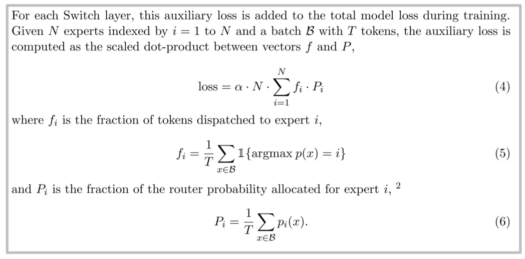
注意loss对$p_i(x)$的梯度为:$\frac{\alpha N}{T^2} \sum 1_{argmax\ p(x)=o}$,这意味着对某个expert更频繁的使用会导致梯度上升,从而对$p_i(x)$本身带来更强的压制(梯度下降更新)。
一个典型例子是switch transformer.
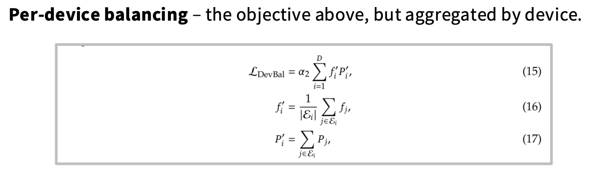
除了上述的per-expert balancing之外,DeepSeek V1-2还引入了per-device balancing,用来平衡不同device之间的负载:
在DeepSeek-V3中,又引入了per-expert biases, 也被称为auxiliary loss free balancing(其实并不能完全做到loss free):
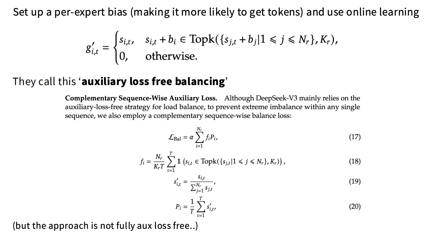
在打分结果上加上一个bias,对于接受token数量超过平均值的expert,降低bias,从而达到负载均衡的效果。
MLA (Multi-Head Latent Attention)
在DS V3中,使用了MLA来做KV状态的压缩。
- 先前的问题是什么?
虽然KV cache这种用空间换时间(存储换计算)的方法,将计算复杂度从$O(N^2)$降低到了$O(N)$,但存在以下问题:
- kv cache的显存大小成为decoding瓶颈;
- 计算量的下降,让decoding过程成为memory bound;
- 为了提高计算强度,BS的增大又受到了1的制约;
所以思考,能否存在一种折中方案?即沿用先前空间换时间的优化思路,但是不要那么激进?可以允许适度提高计算量,但是要进一步压缩KV cache.
一个常用的改变计算强度的优化方法就是利用矩阵结合律,和linear attention类似:
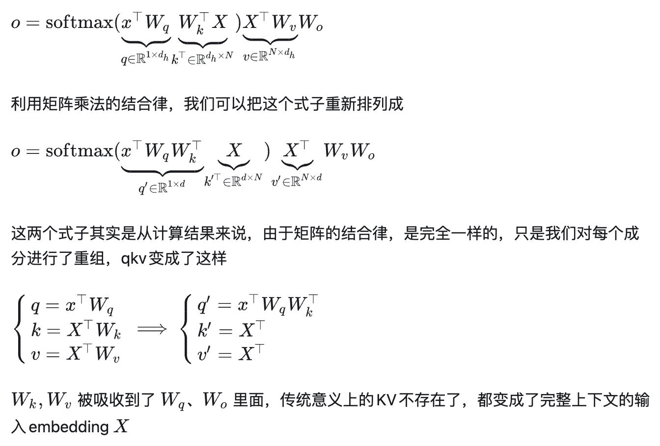
这种方法也被叫做矩阵吸收。经过改造后,原有的KV cache也被替代为:缓存前置的Prefill的$(N\times d)$输入,即$X^T$,$d$为hidden dimension. 优化做到这一步,KV cache的大小已经节省为原本的一半,从$2Nd$降低到$Nd$。
这种方法的副作用是会带来计算量的增加,定量分析后会发现,减少的KV cache比例远低于增加的计算量。所以需要一些技巧来进一步压缩存储:即降维X:
注意到,我们可以把原来的 Key-Value 投影矩阵做低秩分解:
$$W_k' = W_{DKV}W_{UK}$$ $$W'_v=W_{DKV}W_{UV}$$其中:
- \(W_{DKV}\):把输入压缩到较低维的潜向量,便于放入 cache;维度为$(d\times d_c)$
- \(W_{UK}\):再从潜向量恢复出 Key;维度为$(d_c\times d_h)$
- \(W_k'\):两步合起来等价得到的完整 Key 投影矩阵;维度为$(d\times d_h)$
因此图中的注意力分数为$x^\top W_q W_{UK}^\top W_{DKV}^\top X$;再利用矩阵吸收的想法,便得到了压缩后的缓存表示$X^TW_{DKV}$,也就是论文中的$C$,维度为$(N\times d_c)$。之后每次decode再把新的$xW_{DKV}$追加到当前的KV cache内。
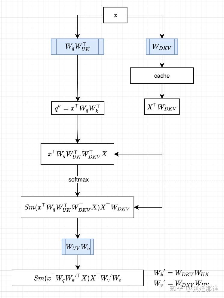
上图中有个小笔误,即左侧$q''$应为$x^TW_qW^T_{UK}$.
这样节省的KV cache比例进一步增大,可以平衡带来的计算开销。
除了在显存制约和计算强度之间取得更好均衡外,矩阵吸收的另一个潜在好处是,假使已知前提是要缓存$C$,矩阵吸收增加的计算复杂度相比于计算$W_k^{'}$和$W_v^{'}$来恢复原本的$K$ $V$矩阵增加的计算复杂度更低。
如果只为了降低显存占用而降维$X$,不做矩阵吸收,那每次恢复完整的$KV$矩阵都需要用缓存的$C$重新做一遍$W^T_{UK}(C)$以及$(C)W_{UV}$,该过程每次所有的历史token都要参与计算,给计算过程增加了$O(Nd_hd_c)$的计算复杂度。通过矩阵吸收,变换后的$q$可以直接和$C$计算,原本$qK^T$的注意力分数计算复杂度为$O(Nd_h)$,现在为$O(Nd_c)$,所以把多出来的计算复杂度降低到了$O(N(d_c-d_h))$,这相比恢复$KV$矩阵要划算的多。
虽然每次变换$q$也会多出来$O(d_h(d+d_c))$的计算复杂度,但是因为是在单token上操作的,所以相比较,计算KV的部分才是大头.
- 为什么training和prefill阶段不需要做矩阵吸收?
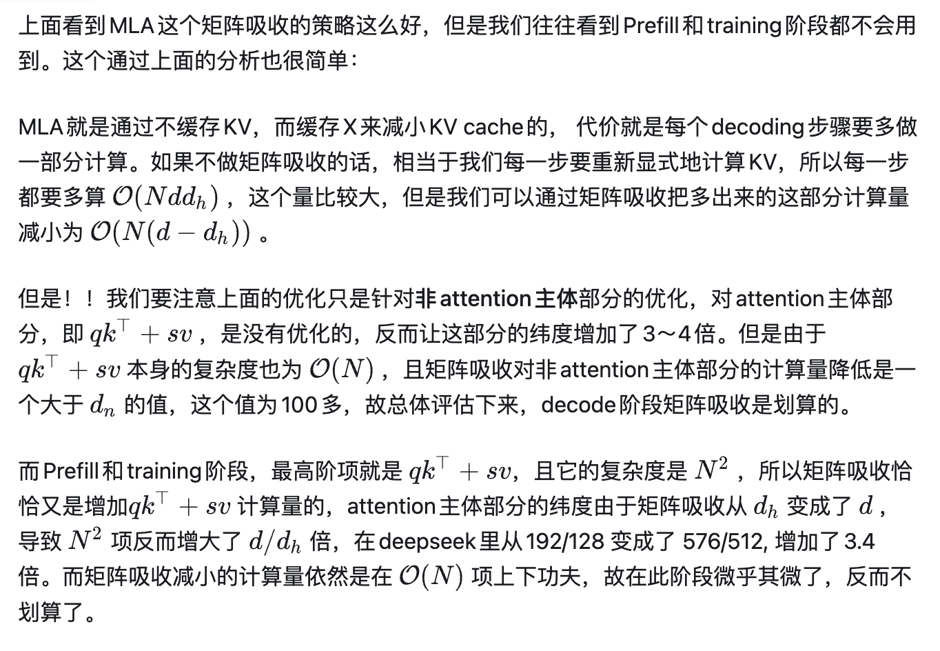
在前边的分析中,我们也看到了,矩阵吸收仅能降低带来的多余的计算复杂度而无法完全避免,在训练和Prefill场景中,多出的计算复杂度变成了平方级,即$O(N^2(d_c-d_h))$,这就不太划算了。所以在训练和prefill阶段,只会做低秩压缩,而不会做矩阵吸收。
- ROPE是如何与MLA共存的?
首先明确,为什么ROPE不能直接应用在MLA上?因为ROPE矩阵是一个和位置相关的矩阵,不是固定的,导致每次新的token都要重新计算,从而降低推理效率。
加入标准 RoPE 后,RoPE 会根据 token 的位置使用不同的旋转矩阵:
$$\tilde q_i=R_iq_i,\qquad \tilde k_j=R_jW^{UK}c_j^{KV}$$注意力分数变为:
$$\tilde q_i^\top\tilde k_j =q_i^\top R_i^\top R_jW^{UK}c_j^{KV}$$这破坏了矩阵吸收的基本形式,每次在计算位置$i$的注意力分数时,还需要使用位置$j$的旋转矩阵,其不能被吸收到固定权重里,也就无从谈起提升推理效率。
解决方法:
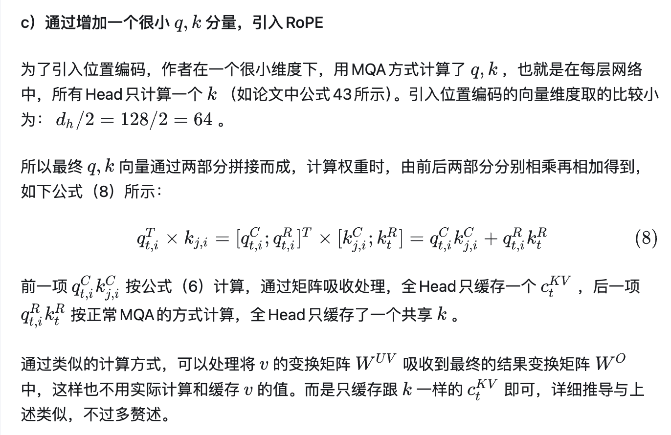
具体参考:
- MLA的问题和优化手段
和普通的MHA不同,MLA类似于GQA,不同的head会共享同一份KV cache;而常规的TP attention因为切分的是head,所以会在各卡中重复缓存同一份KV cache,该问题在MHA中不存在,因为MHA的KV cache本身就按照head区分,所以按照head做TP时,通常可以把KV cache切开。
于是为了节省KV cache显存,DP attention不切heads,切请求。从Prefill开始,每个DP rank就会接受不同请求,从而每个rank上只保留对应请求的KV cache,但是均有全部的heads。
| TP attention:latent每卡复制 | DP attention:请求分卡 | |
|---|---|---|
| 每卡KV cache | N个缓存token*C字节MLA cache | NC/P |
| 全部卡KV cache合计 | P张卡*N个缓存token*C字节MLA cache | NC |
具体可以参考SGLang代码。
MOE stability
other train methods
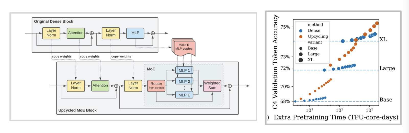
- Upcycling
使用预先训练好的dense模型,load到MOE模型上:
GPUs TPUs
TPU
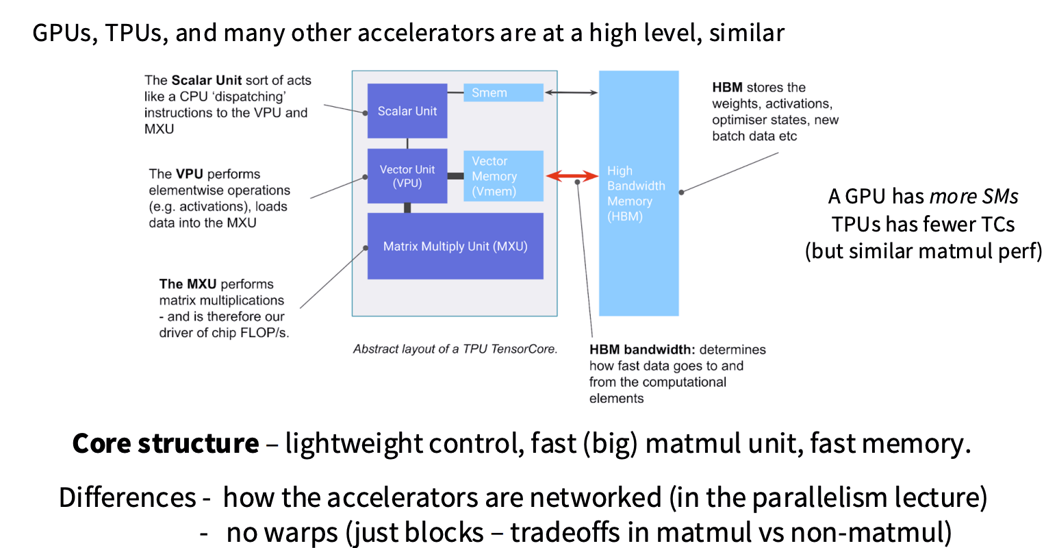
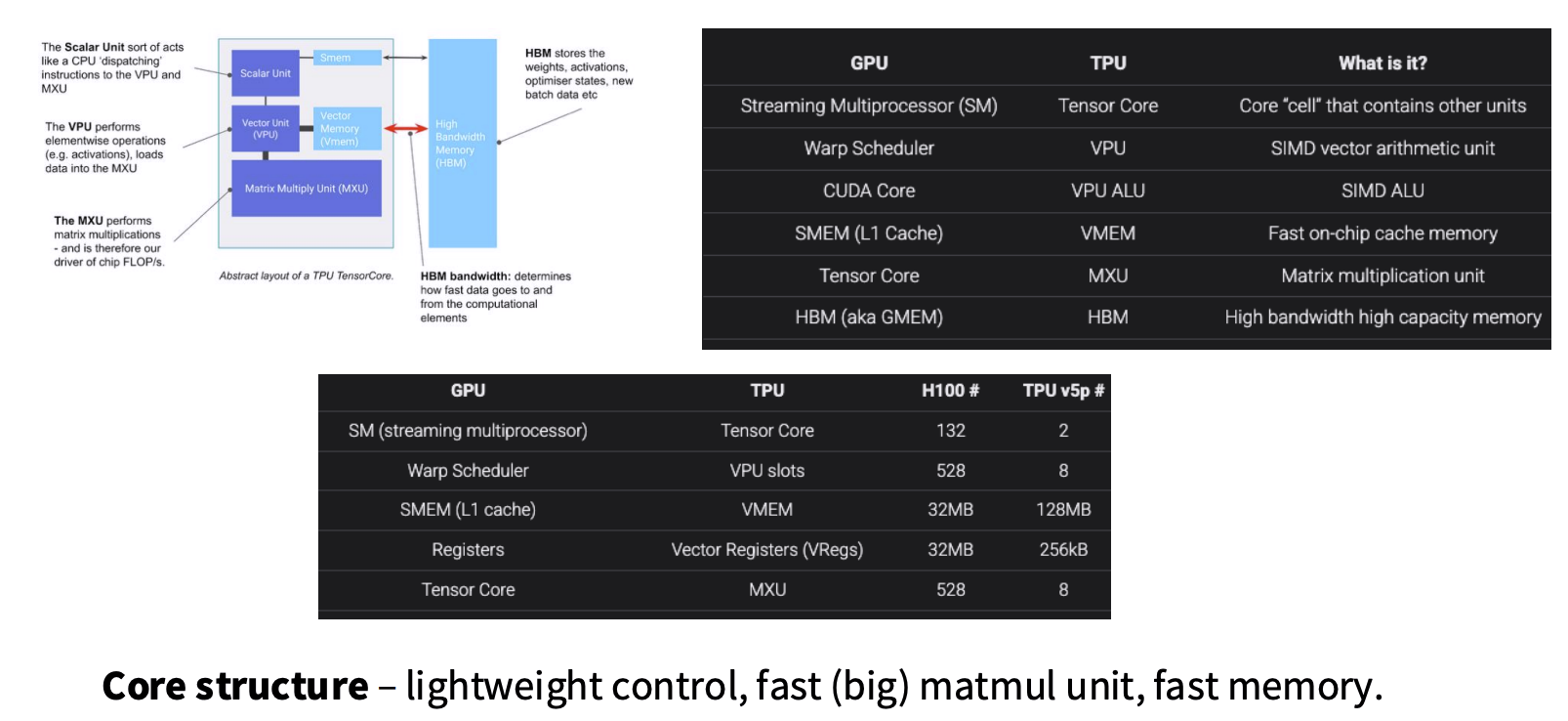
TPU与GPU在很多设计上相似,核心区别在于其处理矩阵乘的单元是一个大单元,而GPU是很多个小的tensor core单元来加速matmul的;同时两者对tensor core的定义不一样。
Making GPUs go fast
这里主要讨论如何优化memory pass。
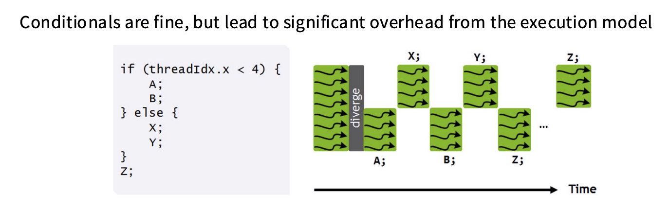
- Control divergence (not a memory issur)
在同一时刻,同一warp中的所有线程处于同一代码段,如果不需要执行对应分支,则等待:
- Low precision computation
可以使用16bit(BF16/FP16)的操作:matrix ops、大部分pointwise操作(relu/add/sub/mul);
需要更高精度(FP32/FP16)的操作:reduction (sum/softmax/norm),因为较小的值累加很容易出现rounding errors;
需要使用更大range(FP32/BF16)的操作:返回结果比输入大很多的pointwise ops (exp, log, pow),比如loss function;
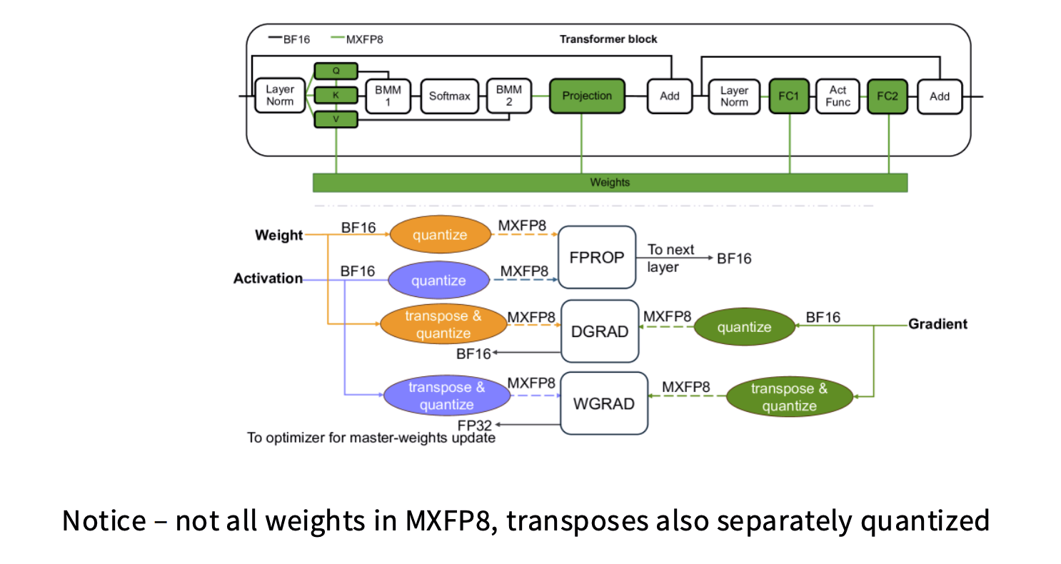
FP8 training:
因为transpose会改变数据排布,需要重新计算scaling,所以MXFP8在内部quantize时,会一次性得到两个矩阵,其中一个用于transpose。
FP4省略。
Operator fusion
recomputation
Memory coalescing and DRAM
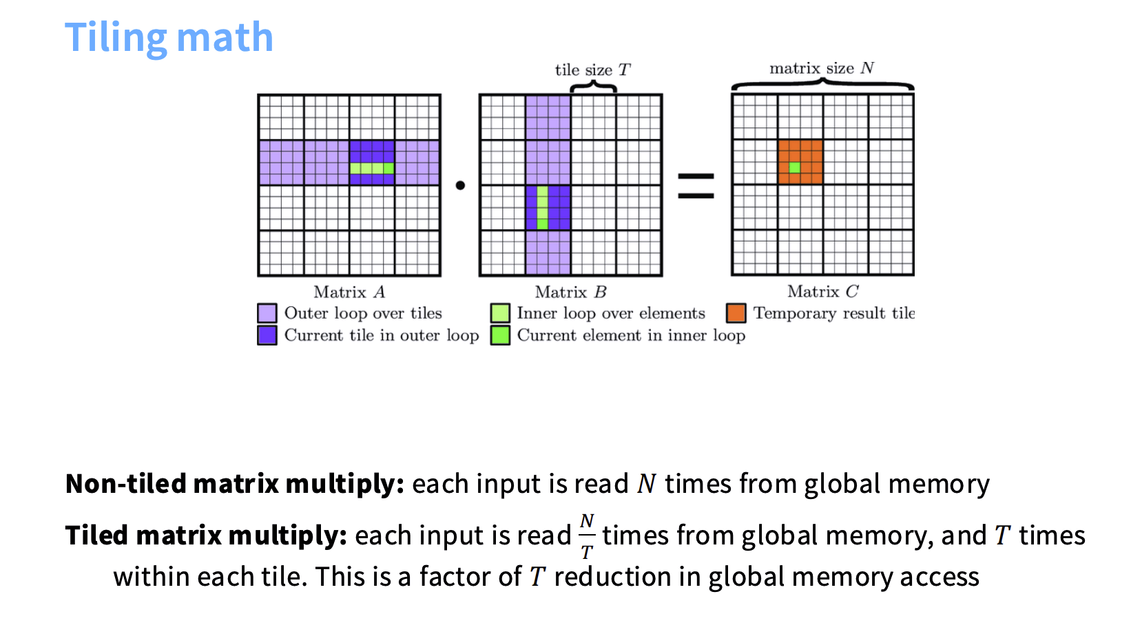
tiling
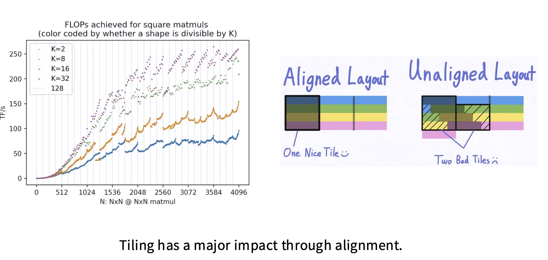
wave quantization
波量化(Wave Quantization):当计算任务超出GPU SM数量时,需要将计算任务分成多个waves进行执行,而这些wave被线性执行需要等待,导致性能下降。
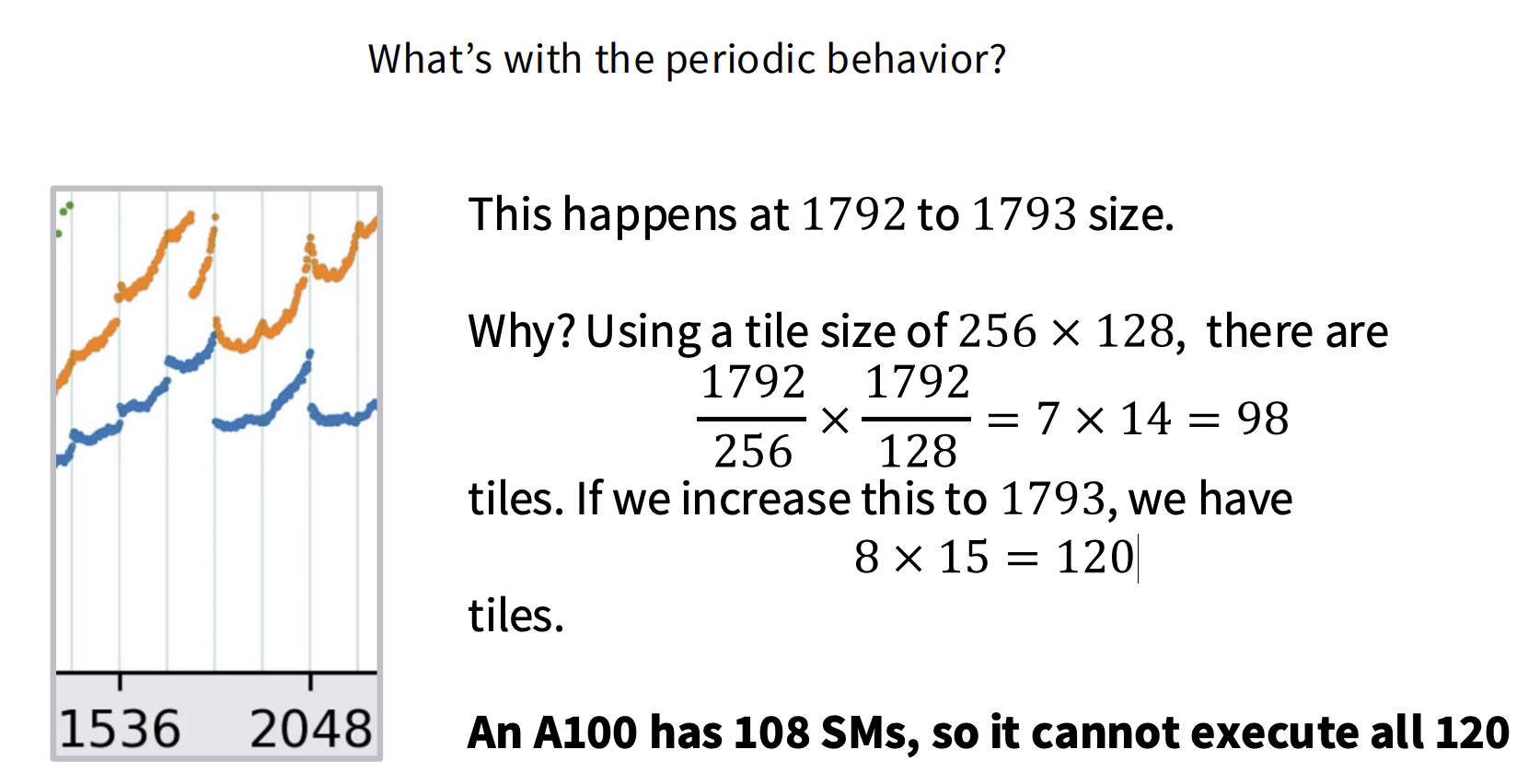
Flash Attention
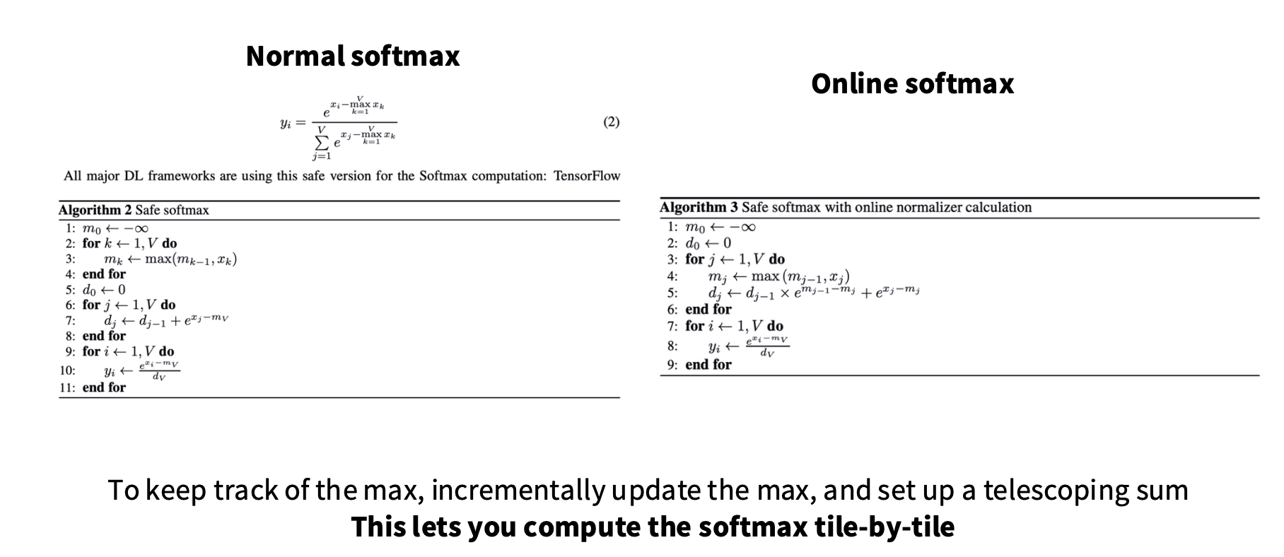
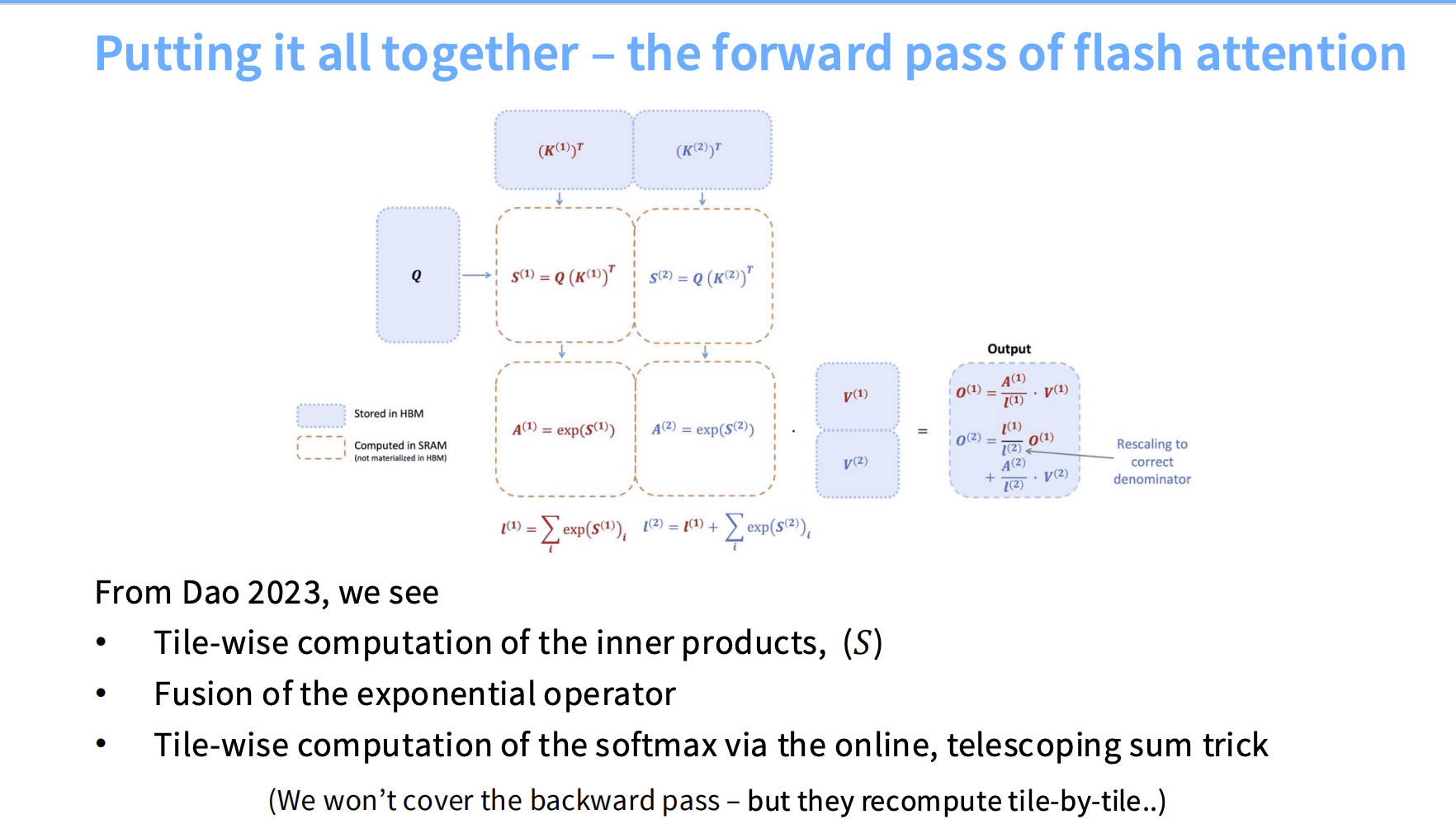
理解从3-pass softmax -> online softmax -> 1-pass flash attention的数学推导:https://zhuanlan.zhihu.com/p/668888063
Kernel, Triton, XLA
kernel basic concepts
一些基本概念。
occupancy
- Each thread can use between 0 and 255 registers.
- The more registers threads use, the fewer threads can be scheduled on an SM (low occupancy).
- Low occupancy isn’t necessarily bad if each thread is doing more work.
- Example: thread coarsening (each thread processes multiple elements).
- Example: thread block has 64 threads, each using 160 registers, SM has 65536 registers
# What we want to run
num_threads_per_block = 128
num_registers_per_thread = 160
# What hardware offers
max_registers = 65536  # Registers allowed per SM
max_warps = 64         # Concurrent warps allowed per SM
# What we can run at once
assert num_registers_per_thread <= 255
num_registers_per_block = num_threads_per_block * num_registers_per_thread
num_blocks = max_registers // num_registers_per_block  # Limited by registers
num_warps = num_blocks * num_threads_per_block / 32
occupancy = num_warps / max_warps
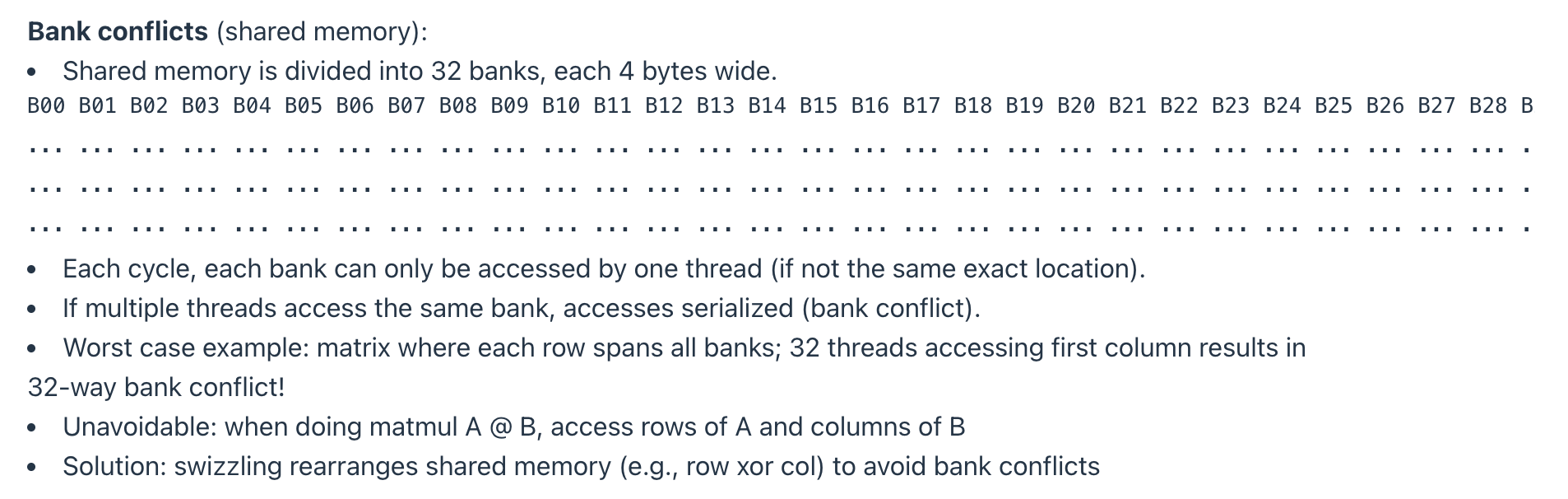
Bank Conflicts
同一个warp中的每个线程对share mem访问的是同一个bank中的地址(不是完全一样的地址,否则会触发broadcast):
Memory coalescing
针对HBM:
When the 32 threads in a warp access HBM, memory accesses combined into transactions of 128 bytes (cache lines).
    M00 M01 M02 M03 M04 M05 M06 M07 M08 M09 M10 M11 M12 M13 M14 M15 M16 M17 M18 M19 M20 M21 M22 M23 M24 M25 M26 M27 M28 M29 M30 M31
    M32 M33 M34 M35 M36 M37 M38 M39 M40 M41 M42 M43 M44 M45 M46 M47 M48 M49 M50 M51 M52 M53 M54 M55 M56 M57 M58 M59 M60 M61 M62 M63

Best case: full coalescing, all threads access the same cache line (32 threads x 4 bytes = 128 bytes).
Block occupancy
Thread blocks scheduled onto SMs in waves.

B200 has 148 SMs, if we launch 160 thread blocks, first wave has 148 blocks, second wave has 12 blocks.

Wave quantization problem: last wave has fewer thread blocks, leaving some SMs idle (low block occupancy).

Solution: make number of thread blocks divide # SMs.
Profiling
torch自带的profiler,示例:
def profile(run: Callable, num_warmups: int = 1):
    # Warmup
    for _ in range(num_warmups):
        run()
    torch.cuda.synchronize()
    # Run the code with the profiler
    with torch.profiler.profile(activities=[ProfilerActivity.CUDA],
            experimental_config=torch._C._profiler._ExperimentalConfig(verbose=True)) as prof:
        run()
        torch.cuda.synchronize()
    # Print out table
    table = prof.key_averages().table(sort_by="cuda_time_total",
                                      max_name_column_width=100,
                                      row_limit=10)
    # Append to profiles.txt
    with open("var/profiles.txt", "a") as f:
        f.write(f"Profile at {time.ctime()}:\n")
        f.write(table)
        f.write("\n\n")
    return table
Triton
指定thread block做什么。
会将数据加载到shared memory中,再写回global memory。
Element-wise example:
@triton.jit
def triton_gelu_kernel(x_ptr, y_ptr, num_elements, BLOCK_SIZE: tl.constexpr):
    # Input starts at `x_ptr`
    # Output starts at `y_ptr`
    # | T T T T T T T T | T T T T T T T T | T T T T T T T T | T T T T T T T T |
    # |    Block 0      |    Block 1      |     Block 2      |    Block 3     |
    pid = tl.program_id(axis=0)      # Identifies the block
    start = pid * BLOCK_SIZE         # Starting index of this block
    # Indices where this thread block should operate
    offsets = start + tl.arange(0, BLOCK_SIZE)
    # Don't read/write past the end of the tensor
    mask = offsets < num_elements
    # Read
    x = tl.load(x_ptr + offsets, mask=mask)
    # Approx gelu is 0.5 * x * (1 + tanh(sqrt(2/pi) * (x + 0.044715 * x^3)))
    # Compute (tl.tanh doesn't exist, use tanh(a) = (exp(2a) - 1) / (exp(2a) + 1)
    a = 0.79788456 * (x + 0.044715 * x * x * x)
    exp = tl.exp(2 * a)
    tanh = (exp - 1) / (exp + 1)
    y = 0.5 * x * (1 + tanh)
    # Store
    tl.store(y_ptr + offsets, y, mask=mask)
triton经过compile后生成PTX.
Row-wise Example:
@triton.jit
def triton_softmax_kernel(x_ptr, y_ptr, x_row_stride, y_row_stride, num_cols, BLOCK_SIZE: tl.constexpr):
    assert num_cols <= BLOCK_SIZE
    # Process each row independently
    row_idx = tl.program_id(0)
    col_offsets = tl.arange(0, BLOCK_SIZE)
    # Read from global memory
    x_start_ptr = x_ptr + row_idx * x_row_stride
    x_ptrs = x_start_ptr + col_offsets
    x_row = tl.load(x_ptrs, mask=col_offsets < num_cols, other=float("-inf"))
    # Compute
    x_row = x_row - tl.max(x_row, axis=0)
    numerator = tl.exp(x_row)
    denominator = tl.sum(numerator, axis=0)
    y_row = numerator / denominator
    # Write back to global memory
    y_start_ptr = y_ptr + row_idx * y_row_stride
    y_ptrs = y_start_ptr + col_offsets
    tl.store(y_ptrs, y_row, mask=col_offsets < num_cols)
如果需要切分tile:
@triton.jit
def row_sum_kernel(x_ptr, out_ptr, N, BLOCK_SIZE: tl.constexpr):
    row = tl.program_id(0)  # Which row are we processing?
    # Accumulator for each thread
    # One row: T1 T2 T3 T4 | T1 T2 T3 T4 | T1 T2 T3 T4 (N = 12, BLOCK_SIZE = 4)
    acc = tl.zeros([BLOCK_SIZE], dtype=tl.float32)
    # Loop over tiles
    for start in range(0, N, BLOCK_SIZE):
        cols = start + tl.arange(0, BLOCK_SIZE)
        mask = cols < N
        x = tl.load(x_ptr + row * N + cols, mask=mask, other=0.0)
        acc += x
    # Final reduction from BLOCK_SIZE (all threads) to a scalar
    result = tl.sum(acc, axis=0)
    tl.store(out_ptr + row, result)
Matmul example:
@triton.jit
def matmul_relu_kernel(
    a_ptr, b_ptr, c_ptr,    # Compute c = a
    M, N, K,                # a is M x K, b is K x N, c is M x N
    stride_am, stride_ak,   # How to navigate a
    stride_bk, stride_bn,   # How to navigate b
    stride_cm, stride_cn,   # How to navigate c
    BLOCK_M: tl.constexpr,
    BLOCK_N: tl.constexpr,
    BLOCK_K: tl.constexpr,
):
    # We are working on the (m, n)-th tile
    pid_m = tl.program_id(0)
    pid_n = tl.program_id(1)
    # Indices
    indices_m = pid_m * BLOCK_M + tl.arange(0, BLOCK_M)  # Row indices of a [BLOCK_M]
    indices_n = pid_n * BLOCK_N + tl.arange(0, BLOCK_N)  # Column indices of b [BLOCK_N]
    indices_k = tl.arange(0, BLOCK_K)                    # Row indices of a = column indices of b [BLOCK_K]
    # Initial matrix of pointers of a and b
    a_ptrs = a_ptr + indices_m[:, None] * stride_am + indices_k[None, :] * stride_ak  # [BLOCK_M, BLOCK_K]
    b_ptrs = b_ptr + indices_k[:, None] * stride_bk + indices_n[None, :] * stride_bn  # [BLOCK_K, BLOCK_N]
    acc = tl.zeros([BLOCK_M, BLOCK_N], dtype=tl.float32)
    # Move along row tiles of a, column tiles of b
    for k in range(0, K, BLOCK_K):
        a = tl.load(a_ptrs, mask=(indices_m[:, None] < M) & (indices_k[None, :] + k < K), other=0.0)
        b = tl.load(b_ptrs, mask=(indices_k[:, None] + k < K) & (indices_n[None, :] < N), other=0.0)
        acc += tl.dot(a, b)
        a_ptrs += BLOCK_K * stride_ak  # Advance to the next row tile of a
        b_ptrs += BLOCK_K * stride_bk  # Advance to the next column tile of b
    # Apply activation function (e.g., ReLU)
    acc = tl.maximum(acc, 0.0)
    # Write output tile
    c_ptrs = c_ptr + indices_m[:, None] * stride_cm + indices_n[None, :] * stride_cn
    tl.store(c_ptrs, acc, mask=(indices_m[:, None] < M) & (indices_n[None, :] < N))
这行代码将1d的indice_m和indice_k通过broadcast,变成2d的shape:
a_ptrs = a_ptr + indices_m[:, None] * stride_am + indices_k[None, :] * stride_ak
Parallelism
DP
为什么DP不够用?
因为随着机器数量的增加,首先每个节点上的样本不能太少,否则通信开销占比过大;其次如果每个机器上样本过多,如果超过critical batch size,在batch梯度中,从噪声(variance)主导区进入有效梯度信号主导区,梯度已经比较准确,那么继续增大batch,收敛速度不会线性增长,在model scaling law的章节也有讨论:
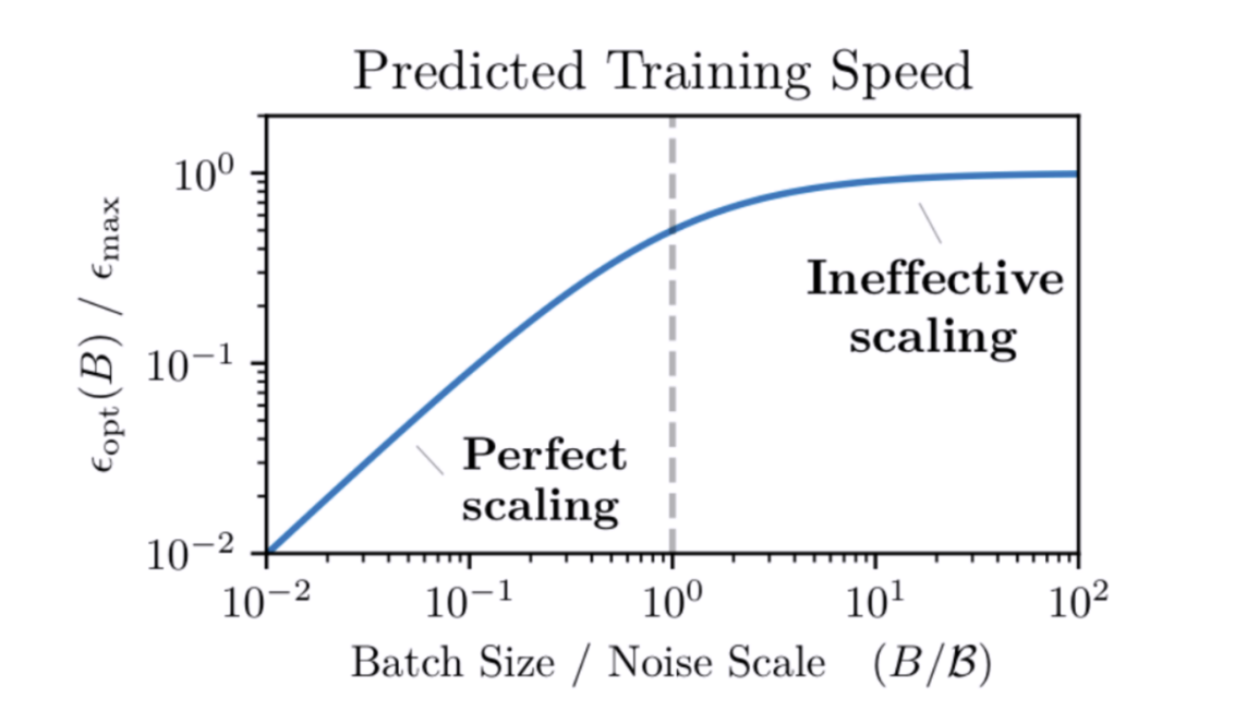
这块关于信噪比的分析可以参考OpenAI的文章:
An Empirical Model of Large-Batch Training: https://arxiv.org/pdf/1812.06162
Zero系列显存策略优化
Zero有两篇论文值得一读,一个是deepspeed原始的Zero论文,首次提出了zero1,2,3的架构,还有一篇论文是Meta PyTorch团队在FSDP上的工作,偏工程实践一些。这里把两篇论文的解读也放在这里:
ZeRO: Memory Optimizations Toward Training Trillion Parameter Models
- 问题1: 显存占用是如何分配的?
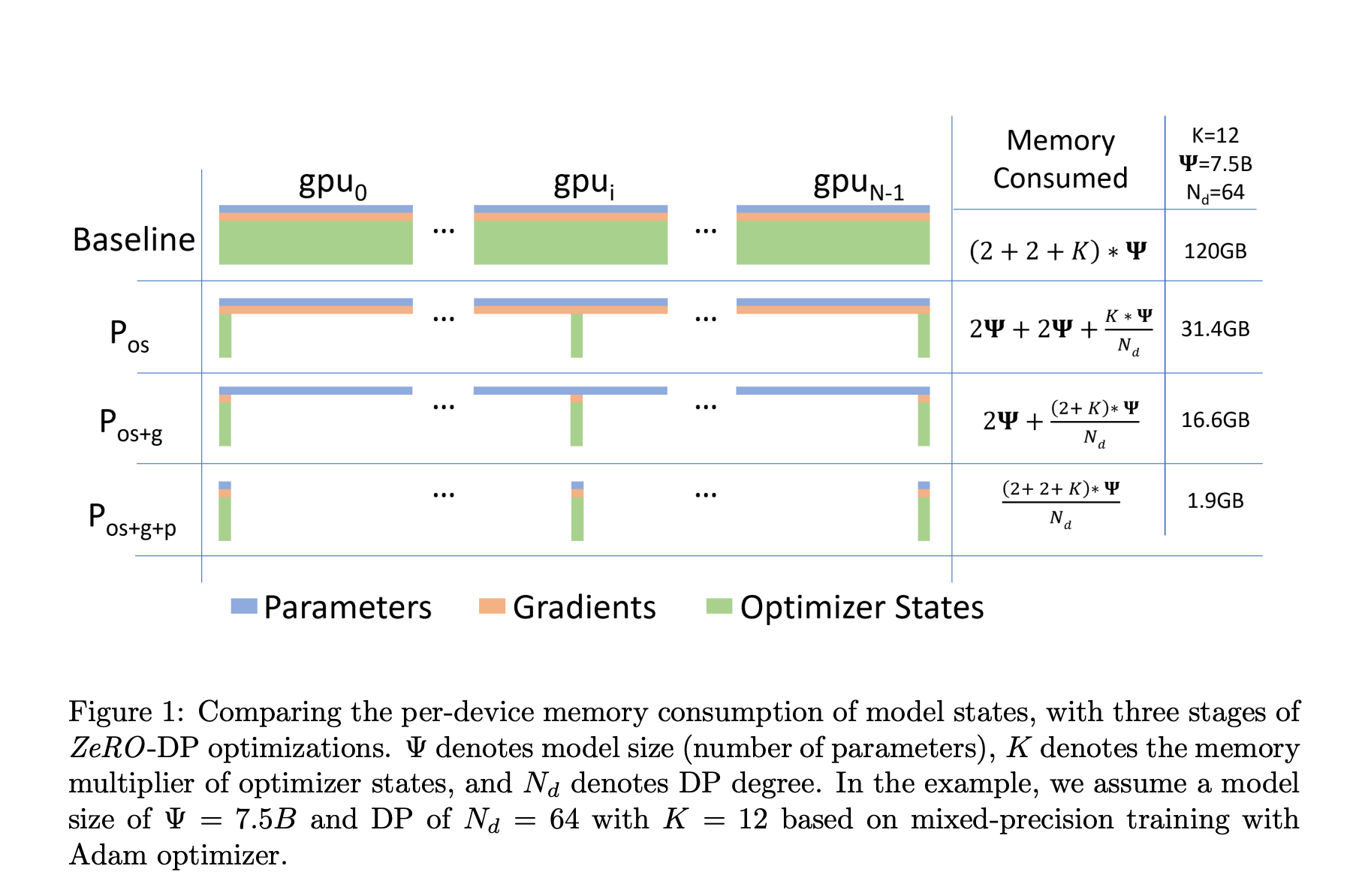
在常见的混精度训练中,一般分为如下几份:bf16的参数+bf16的梯度+fp32的M/V (对于Adam优化器)+fp32的参数拷贝,大概是2+2+12=16的显存占用;
- 问题2: zero的三个阶段分别是什么?
- Zero1: 分片optimizer状态
- Zero2: 分片梯度
- Zero3: 分片参数
通过上边对显存的占用分析,我们可以知道这几种方案对显存的节省程度如下图:
- 这几种不同的zero策略,对通信的开销是多大?
这也是整个zero系列最关键的问题。
要讲明白这个问题,我们要先从DDP开始,DDP的allreduce的通信开销是多大?
参考文章:https://zhuanlan.zhihu.com/p/504957661
- 如何提高通信效率?
做梯度分桶,每个worker负责几个bucket(layers),由于我们可以根据网络梯度计算顺序对梯度bucket做拓扑排序,每个worker上的计算图均按此执行,我们可以在每个worker上的属于shard i的梯度ready之后,参与将梯度reduce到shard i的reduce scatter(当然有的worker reduce scatter的早,有的晚,取决于对应worker分到的bucket位于拓扑图中的哪个位置)。
这样做的好处在于
- 每个worker处理完不属于自己的bucket的梯度之后就可以将其丢弃,节省显存;
- 更好的通信 计算overlap;
allreduce通信开销
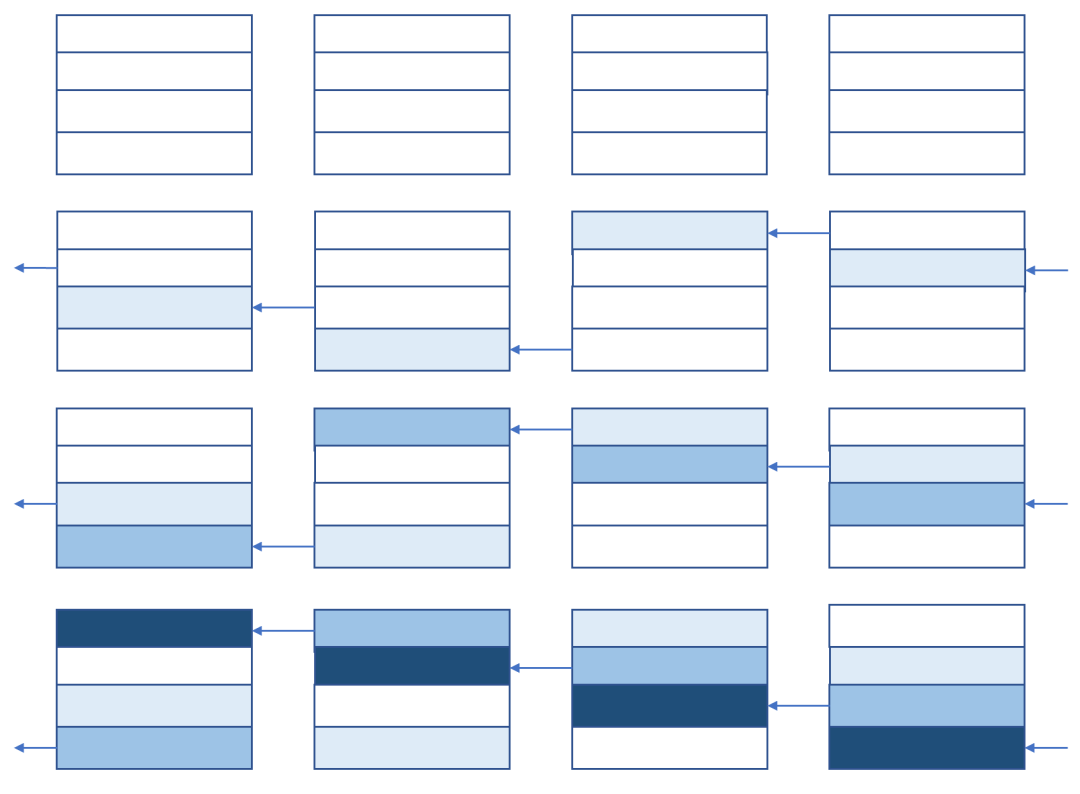
当前最先进的allreduce通信通过两阶段完成:reduce-scatter + all-gather;即每个shard将收到所有属于自己这部分的梯度, 在本地加好,再通过一个allgather让其他所有shard也能收到自己加好的这一份,最终每个shard上都保留了完整的做了reduce-sum的整体梯度。这两个操作均可以通过环形通信算法实现(Ring-Allreduce),具体流程可以看上边贴的知乎链接,结论很重要:
对于p个设备,大小为V的矩阵(每个设备上都有大小为$V$的矩阵,并且被划分成了$p$份);假设双工通信,出入口带宽均为$\beta$,
- 所有设备之前传输的总数据量为$2\times (p-1)v/p\times p=2\times (p-1)\times v$,如果p足够大,近似于$2\times pv$.
- 因为在同一轮内,每个设备在发送数据的同时也可以收到数据,整个过程需要的时间是$2(p-1)v/2p\beta$,如果p足够大,近似于$v/\beta$,与设备数无关;
我们这里的通信时间只考虑传输带宽,而没有考虑每次传输都包含的延迟(latency)。当数据量V比较大时,延迟项可以忽略,上文的分析就是成立的。当 V 特别小,或者设备数 p 特别大时,带宽就变得不重要了,反而是延迟比较关键,这时更好地实现就不是环状算法了,而应该使用树状通信。
这也是为什么英伟达 NCCL 里既实现了ring all-reduce,也实现了 double-tree all-reduce 算法.
因为我们这里要对比的就是allreduce本身带来的通信开销,假定设备数量为常量,那么allreduce的通信开销和v成正比。
Zero1: 在做参数更新后,由于每个worker只存了属于自己的那份优化器状态,所以先做一次reduce_scatter让每个worker收集自己opt分片需要的梯度,做完参数更新后,再通过一次allgather收集更新后的参数就好,这和原本的allreduce无异;通信开销仍为2pv;
Zero2: 每个worker只存自己的优化器状态+梯度,这要求我们
incrementally goes backward on the computation graph:每个worker在计算好某个layer的梯度后,就参与将这份梯度reduce到正确的worker上,之后如果不再需要这份梯度,就立刻free(相当于将一个大的reduce-scatter过程拆分);最后仍然是再做all-gather收集更新后的参数;可以看到,通信开销和先前仍无区别;虽然这里和DDP一样也是reduce_scatter+all_gather,但是这里all_gather的是参数,而非梯度;梯度已经是通过reduce_scatter之后分片的了
Zero3: 每个worker保存自己的优化器状态+梯度+参数,这要求我们在前向和反向都添加额外的通信操作:在前向计算前,通过一次allgather收集参数:为了计算通信的overlap,我们仍然采用分桶策略,总通信开销为$v/p*p*p$;这样的allgather操作在反向也有一个,同时再加上梯度的reduce scatter,总共需要3pv的通信,也即正常方案的1.5倍;
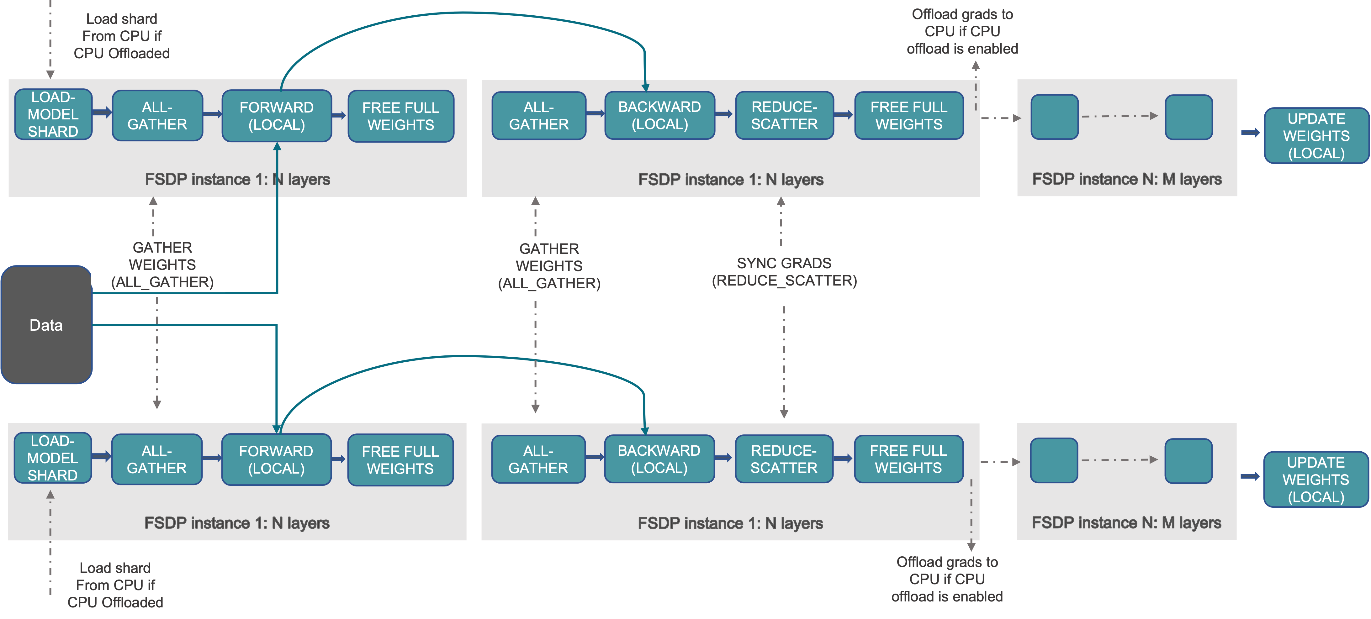
PyTorch FSDP: Experiences on Scaling Fully Sharded Data Parallel
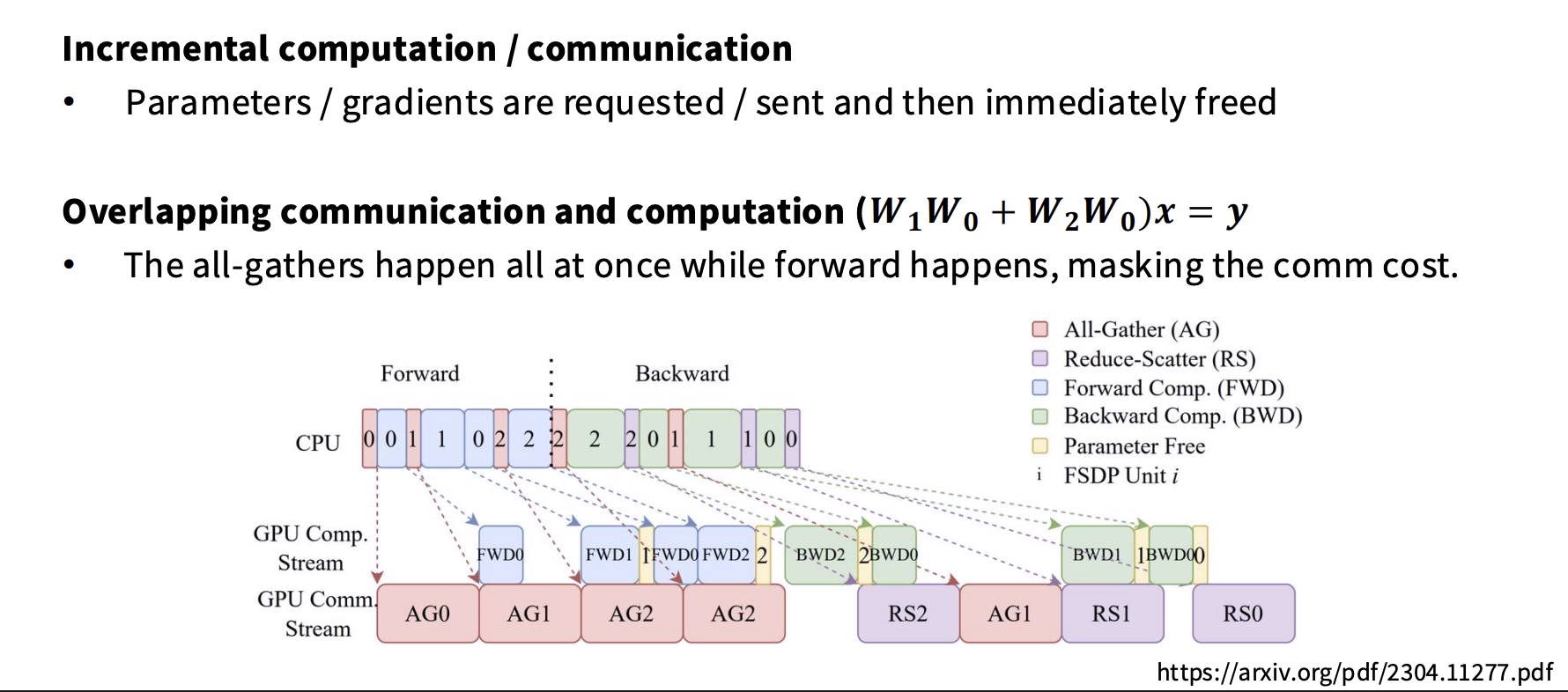
待补充。
TP
def tensor_parallelism_main(rank: int, world_size: int, data: tensor, num_layers: int):
    setup(rank, world_size)
    data = data.to(cuda_if_available(rank))  # All ranks get the data (batch_size x num_dim)
    batch_size = data.size(0)
    num_dim = data.size(1)
    local_num_dim = int_divide(num_dim, world_size)  # Shard `num_dim`
    # Create model (each rank gets 1/world_size of the parameters)
    #  |  |  |  |
    # W0 W1 W2 W3
    #  |  |  |  |
    params = [get_init_params(num_dim, local_num_dim, rank) for layer in range(num_layers)]
    # Forward pass
    x = data
    for layer in range(num_layers):
        # Compute activations (batch_size x local_num_dim)
        x = x @ params[layer]  # Note: this is only on a slice of the parameters
        x = F.gelu(x)
        # Allocate memory for activations (world_size x batch_size x local_num_dim)
        activations = [torch.empty(batch_size, local_num_dim, device=cuda_if_available(rank)) for _ in range(world_size)]
        # Send activations via all gather
        dist.all_gather(tensor_list=activations, tensor=x, async_op=False)
        # Concatenate them to get batch_size x num_dim
        x = torch.cat(activations, dim=1)
    print(f"[tensor_parallelism] Rank {rank}: forward pass produced activations {summarize_tensor(x)}", flush=True)
    # Backward pass: homework exercise
    cleanup()
TP常在一个节点内部,因为需要比较重的通信操作。但是对于TPU而言,因为其采用mesh的方法链接,所以不同节点之间的通信开销差异不大,从而可以使用比较大的TP size。
TP通信流程参考Megatron-LM论文,对于transformer结构,FFN和self-attention各需要两次allreduce(forward+backward),即对于一个transformer layer,需要4次allreduce。
FFN使用allreduce是因为FFN有两层matmul,都做了TP切分,所以实质上形成了:
对第一层linear,因为后续
GeLu不满足线性叠加性,所以要对第一层权重矩阵$A$按照column-parallel切分为$[A_1,A_2]$,输入$X$不需要切分,做$XA$即可。第二层linear为了接上第一层output $Y$,所以对第二层权重矩阵$B$按
row-parallel切分为$[B_1,B_2]^T$,做$YB$。那么,$[Y_1, Y_2] @ [B_1, B_2]^T=Y_1B_1+Y_2B_2$,这个加法就是
allreduce的来源。Self-attention使用allreduce也是因为在attention结构之后接了一个矩阵乘,QKV结构切分时也按照
column-parallel切分,原因是要保证每个head对应的计算都在同一节点上。与上述两者不同的就是对embedding的切分,因为这里不存在两层linear等类似结构,所以只需要一次
AllGather将结果聚合就好,反向对应的就是Reudce-Scatter。
activation analysis
参考:https://proceedings.mlsys.org/paper_files/paper/2023/file/80083951326cf5b35e5100260d64ed81-Paper-mlsys2023.pdf
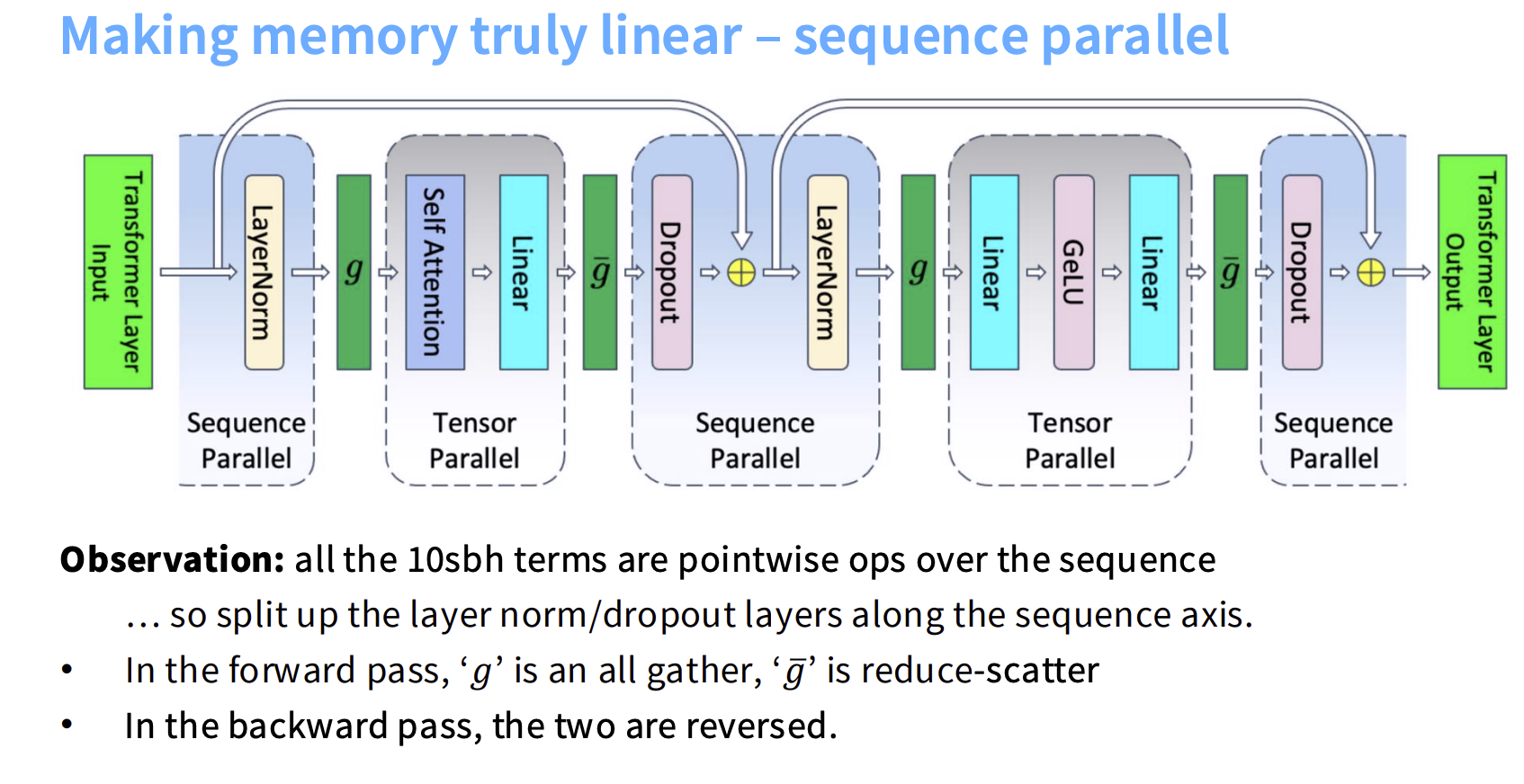
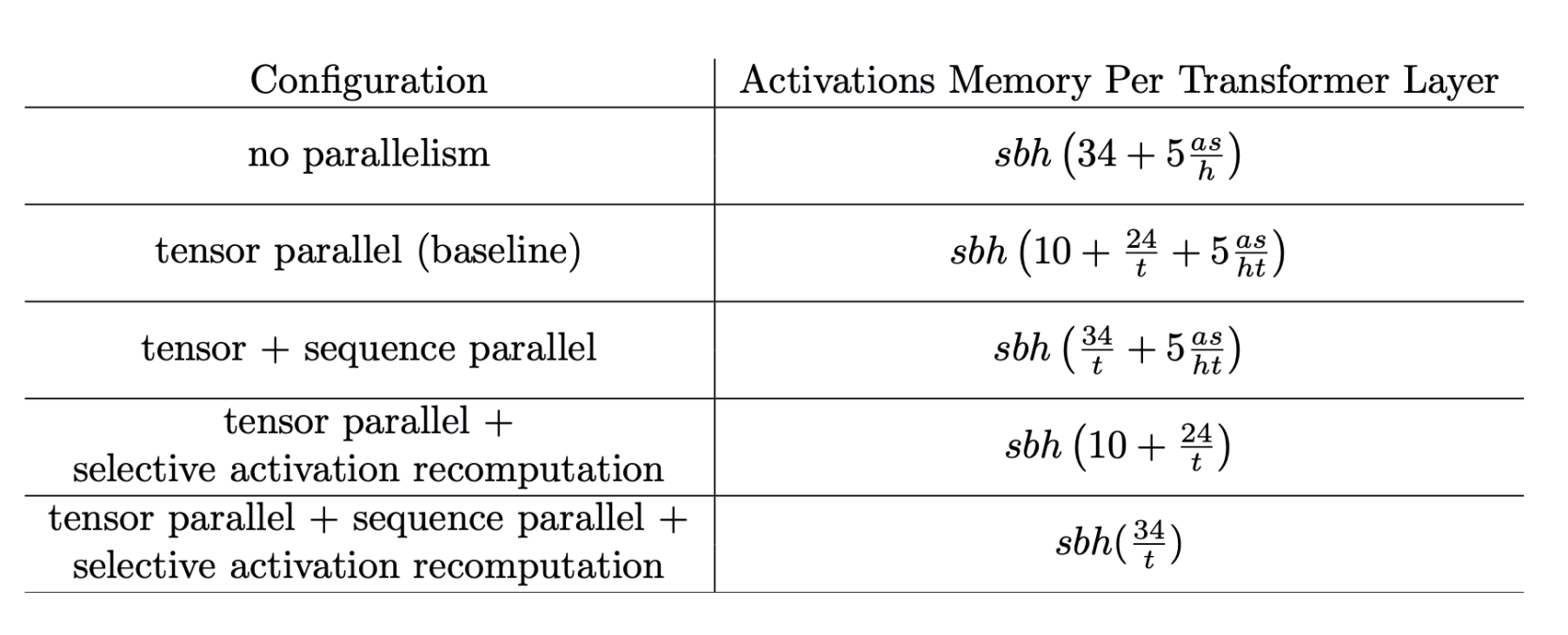
在加上TP之后,activation的大小从$sbh(34+5\frac{as}{h})$–>$sbh(10+\frac{24}{t}+5\frac{as}{ht})$,其中仍然有一个10的常数项不被tensor parallel size影响,它包含了:
- LayerNorm (4bsh)
- Dropout (2bsh)
- Inputs to attention and MLP (4bsh)
这就是为什么我们需要SP (sequence parallel)来切分这些结构。
PP
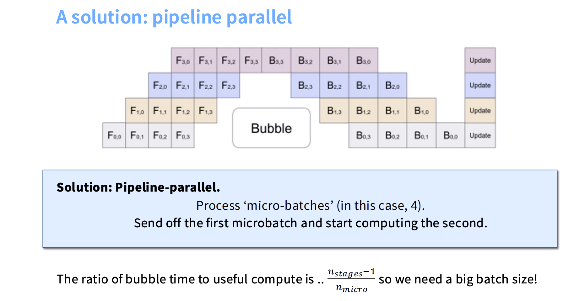
pipeline parallel的好处在于,通信量比较小,基本是activation($B\times S \times H$),而非all-to-all通信,所以比较适合作为最外层的切分组织(在data center或者pod间做PP切分)。
def pipeline_parallelism_main(rank: int, world_size: int, data: tensor, num_layers: int, num_micro_batches: int):
    setup(rank, world_size)
    # Use all the data
    data = data.to(cuda_if_available(rank))
    batch_size = data.size(0)
    num_dim = data.size(1)
    # Split up layers
    local_num_layers = int_divide(num_layers, world_size)
    # Each rank gets a subset of layers
    local_params = [get_init_params(num_dim, num_dim, rank) for layer in range(local_num_layers)]
    # Forward pass
    # Break up into micro batches to minimize the bubble
    micro_batch_size = int_divide(batch_size, num_micro_batches)
    if rank == 0:
        # The data
        micro_batches = data.chunk(chunks=num_micro_batches, dim=0)
    else:
        # Allocate memory for activations
        micro_batches = [torch.empty(micro_batch_size, num_dim, device=cuda_if_available(rank)) for _ in range(num_micro_batches)]
    for x in micro_batches:
        # Get activations from previous rank
        if rank - 1 >= 0:
            dist.recv(tensor=x, src=rank - 1)
        # Compute layers assigned to this rank
        for param in local_params:
            x = x @ param
            x = F.gelu(x)
        # Send to the next rank
        if rank + 1 < world_size:
            print(f"[pipeline_parallelism] Rank {rank}: sending {summarize_tensor(x)} to rank {rank + 1}", flush=True)
            dist.send(tensor=x, dst=rank + 1)
最简单的做法:切分micro-batch之后,按照顺序做1F1B,这是GPipe的方法:
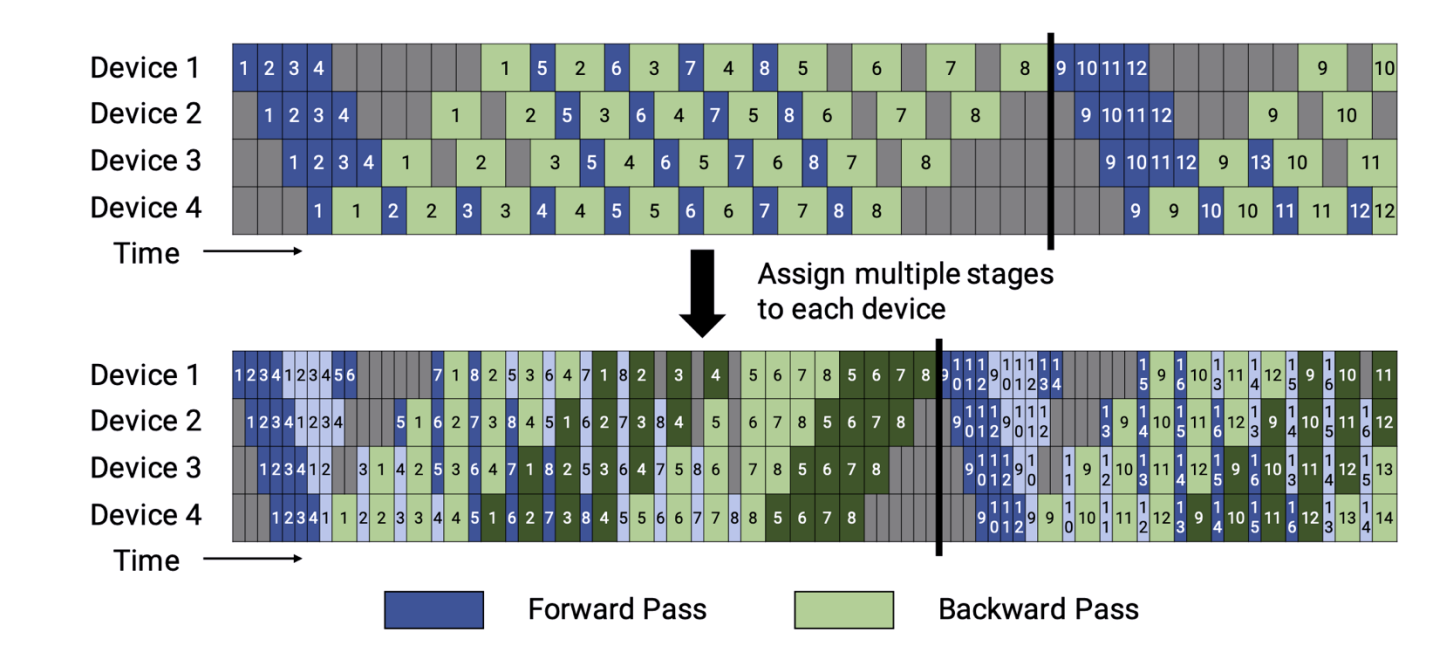
进一步,可以将forward pass和backward pass交叠,即interleave 1F1B:
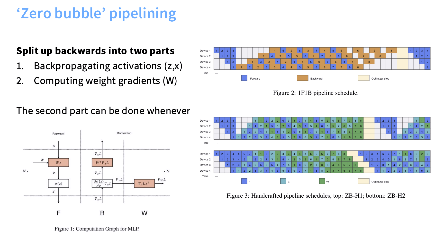
再之后可以考虑反向需要对$W$和输入$X$都做更新,而后者的更新对反向的推动不可或缺,所以可以在空泡中插入对$W$的更新,做成zero-bubble pipeline parallel.
SP
从sequence axis切分而非hidden axis。仍然参考TP部分activation analysis的章节。
EP
EP在MOE场景下比TP好的原因:
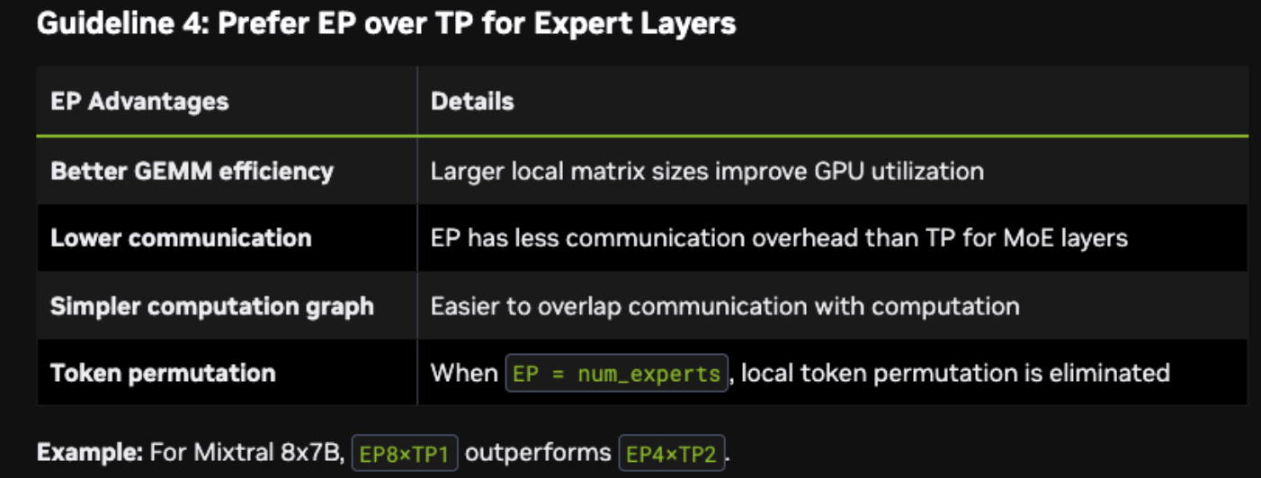
尤其是TP会破坏大矩阵乘。
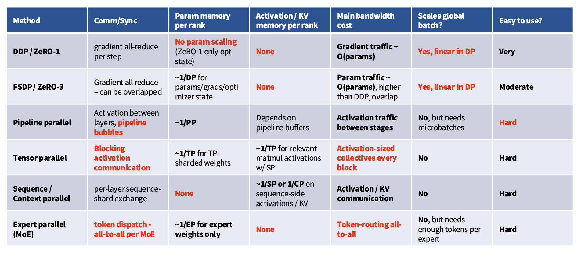
但是在transformer中使用EP时,因为attention本身会使用TP做切分,所以实际上需要对attention和MLP着两个结构的并行策略做解耦:对attention使用high TP,MLP使用EP(low TP).
Scaling Laws
在实际做pre-train时,因为每家的训练配置差别比较大,所以往往无法直接利用现有的scaling law analysis结果(比如chinchilla rule),需要自己做一遍分析(比如Stepfun、DeepSeek、MiNiCPM都做了类似的事情)。
Data Scaling Laws
dataset size -> error
Loss and dataset size is linear on a log-log plot:
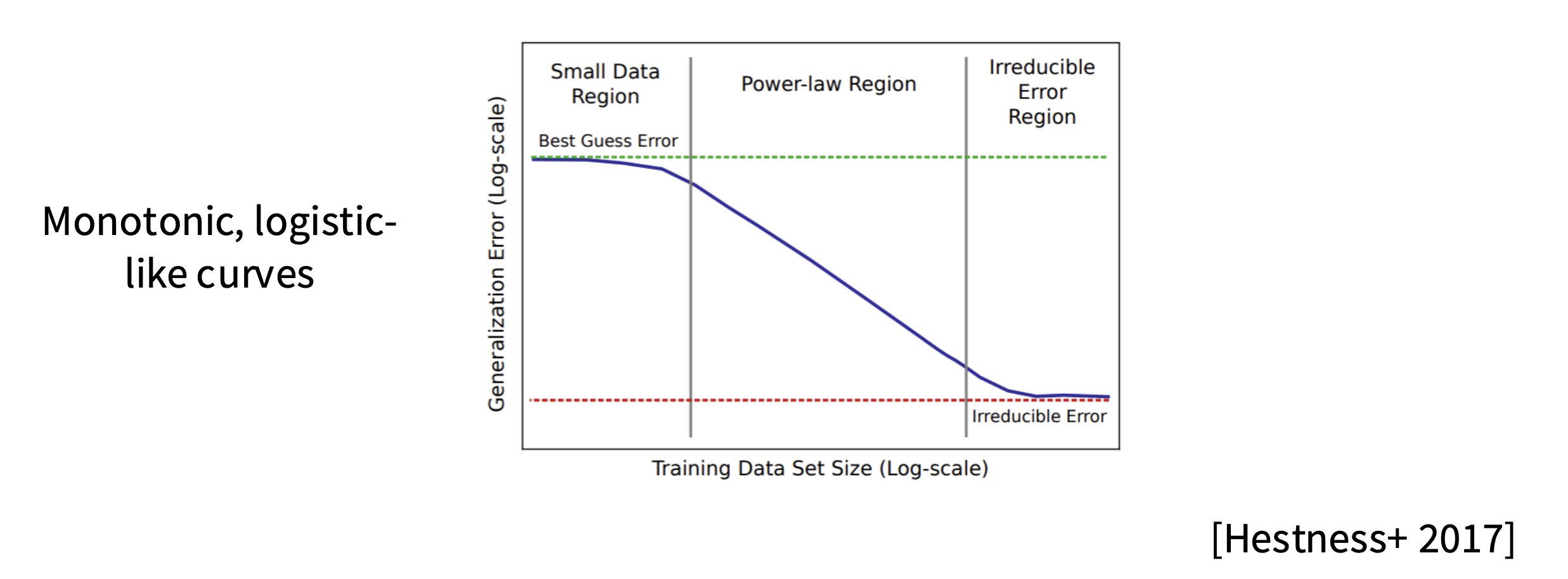
上图表明,Estimation error naturally decays polynomially.
一些类似的例子是mean estimation,以及参数化估计(即对分布有先验假设的学习),error function和$-logn$成线性关系,即$\frac{1}{n}$ Scaling (n为样本数量):
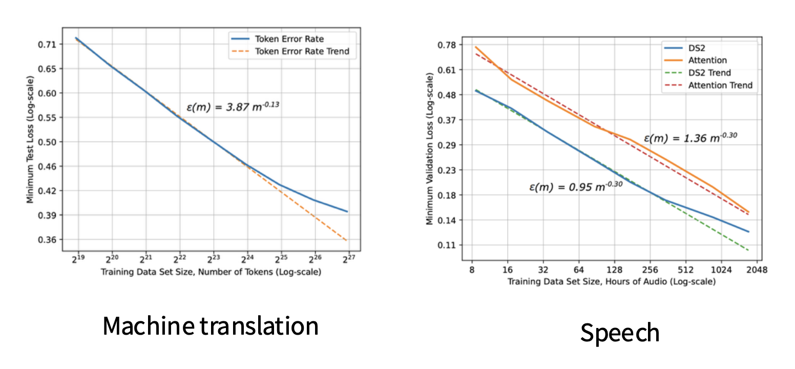
对于语言模型等非参数化(nonparametric)估计,则是和$-\alpha logn$成线性关系,即$\frac{1}{n^\alpha}$ scaling:
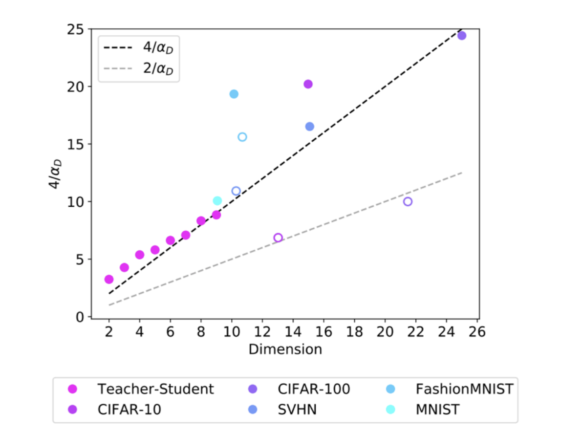
- Scaling laws arise due to polynomial rates of learning $\frac{1}{n^\alpha}$
- Some argue the slope $\alpha$ is closely connected to the intrinsic dimensionality of the data (not always true)
Data composition
影响interception,但是不影响slope:
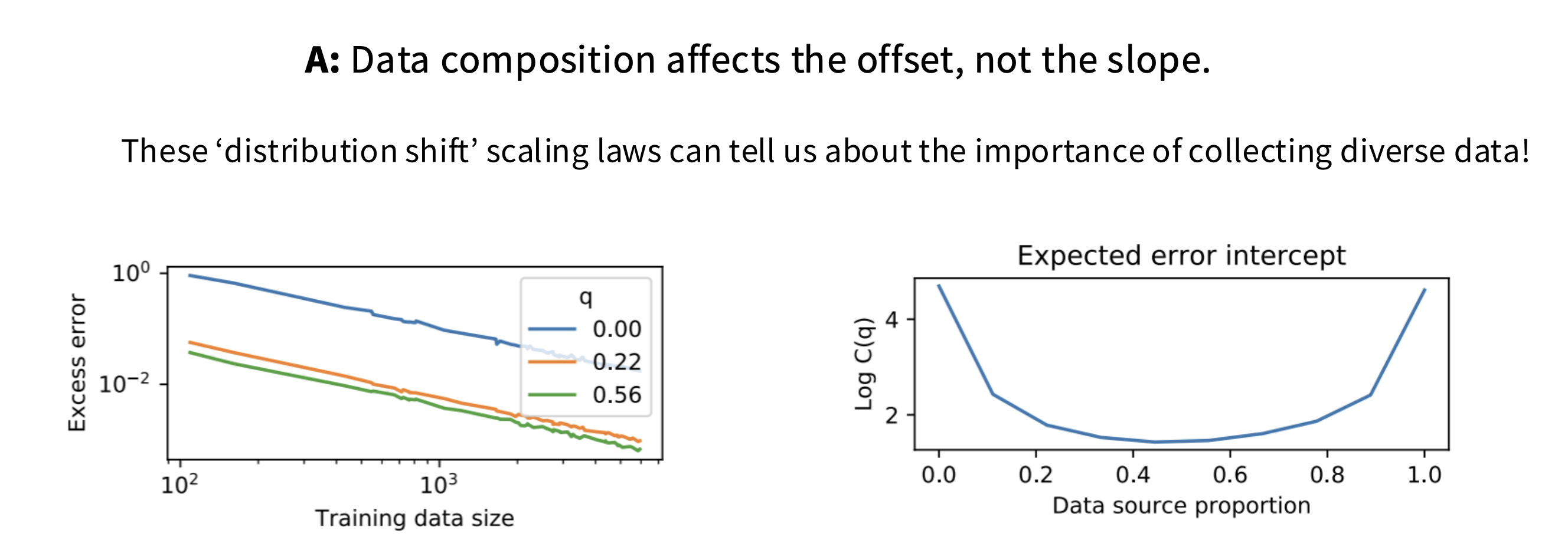
在实际应用中,一般都会直接在小模型上尝试不同的data mixture,然后选择效果最好的直接推广到大模型上(因为只改变distribution shift),而不需要再对新选择的composition验证scaling law效果。
Data repitition
一昧地重复数据会导致scaling law失效;另一方面,我们所讨论的scaling law本身只是模型效果的下界,在对数据配方做更改之后很可能会训练的更好:
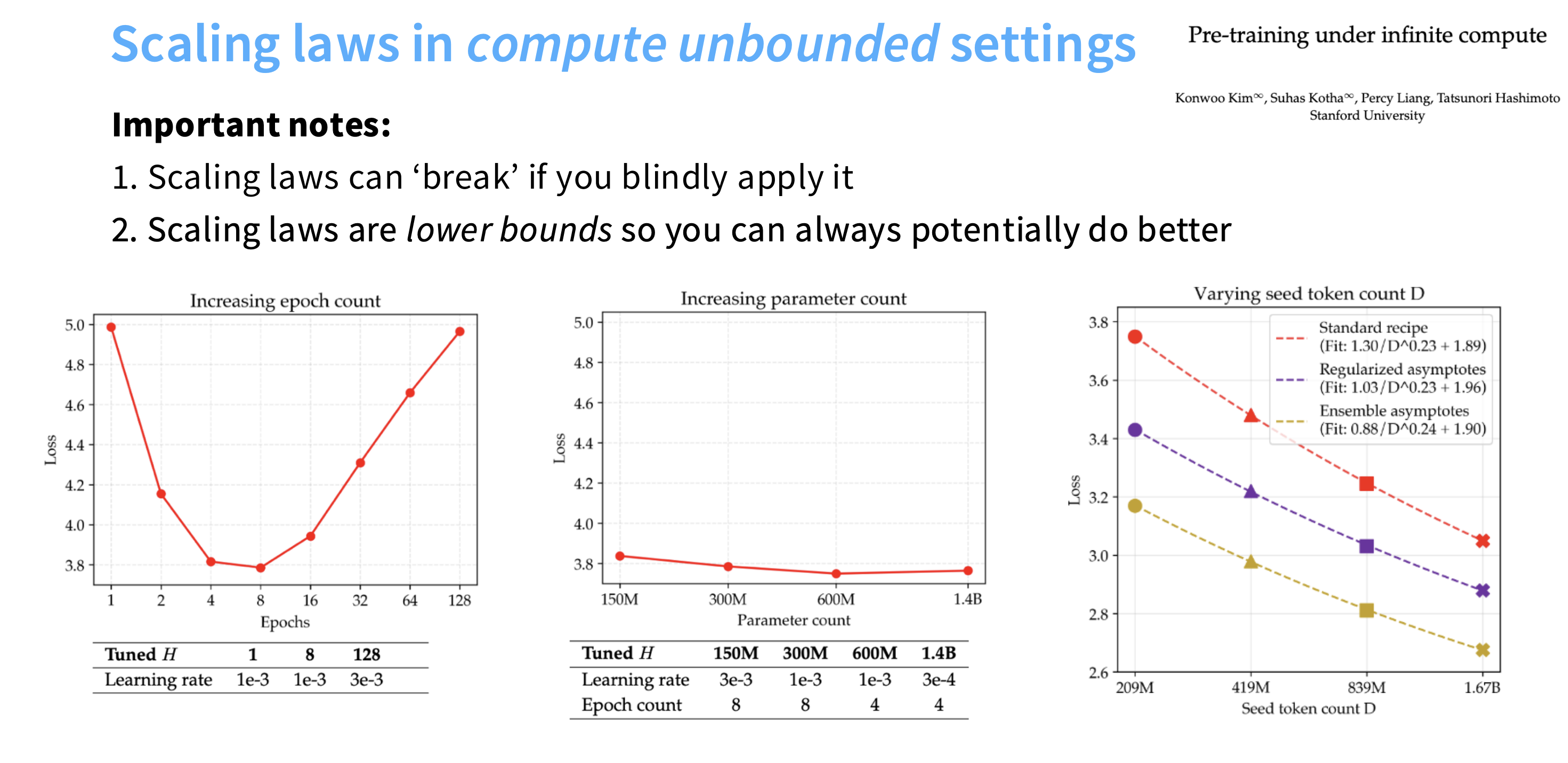
总之,数据的选择会随着算力需求而改变,不是固定的,应当具有适应性。
Model Scaling Laws
从以下五个方面考虑:
- Architecture
要达到相同效果的GPT-3, 训练LSTM要比transformer耗费更多参数;所以transformer效果更好;
- Optimizer
Adam的效果要比SGD更好。
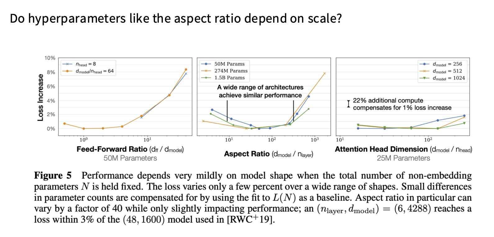
- Aspect ratio / depth
- 层数太少,对效果影响很大
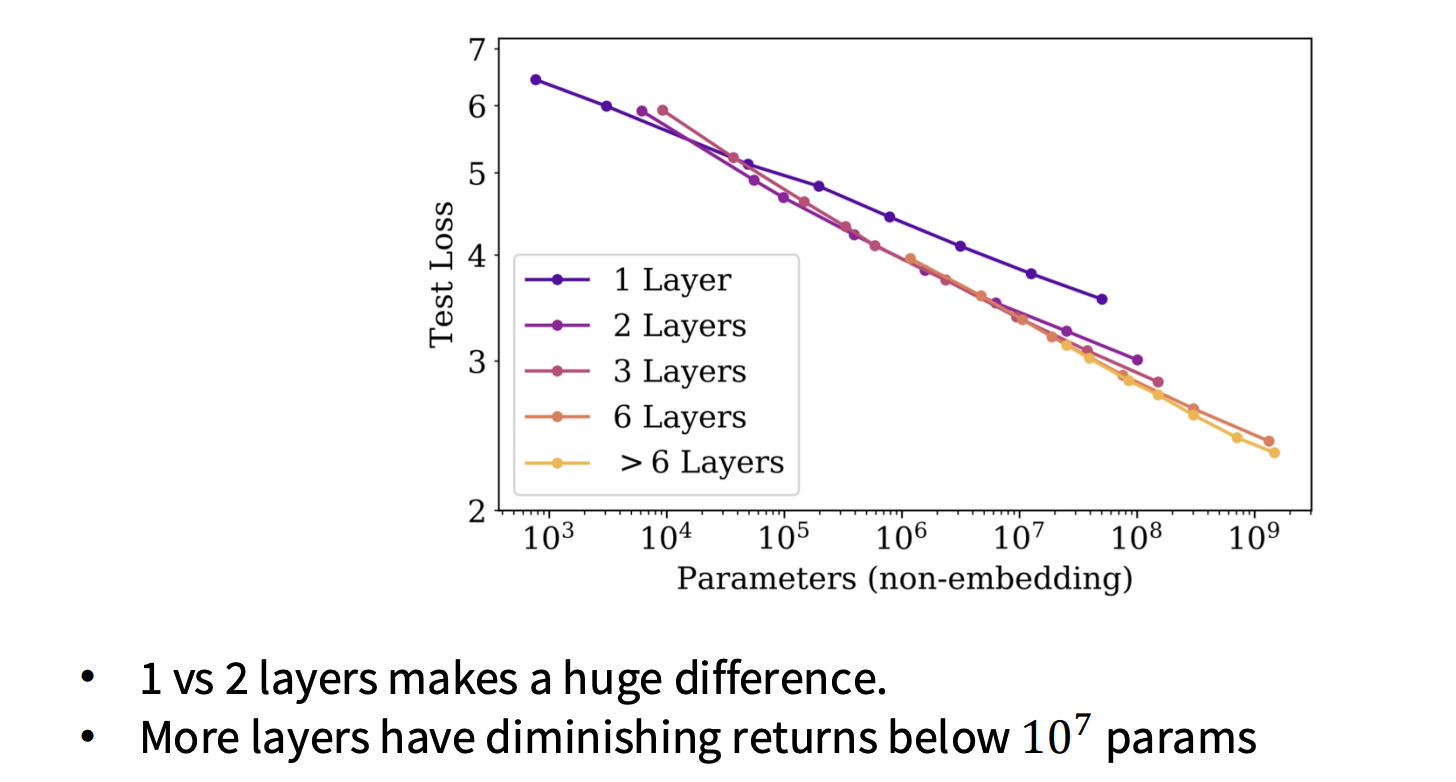
- aspect ratio以及attention head dimension的最优值基本不跟随参数量改变
- 但对
parameter的定义范围会改变scaling law:比如是否包含embedding layer层的参数,
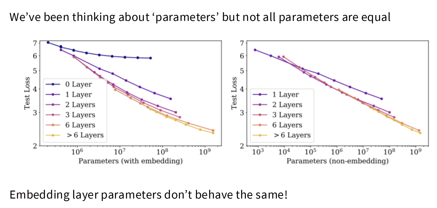
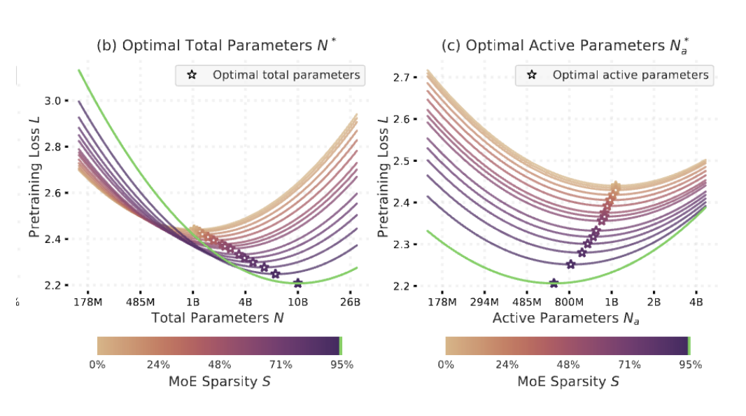
以及对于MOE,active parameter和total parameter的scaling law表现也不同:
- MOE稀疏度越高,达到最好效果需要的active parameters越多;
- MOE稀疏度越高,达到最好效果需要的total parameters越少;
- Batch size
也就是之前在DP章节提到的critical batch size.
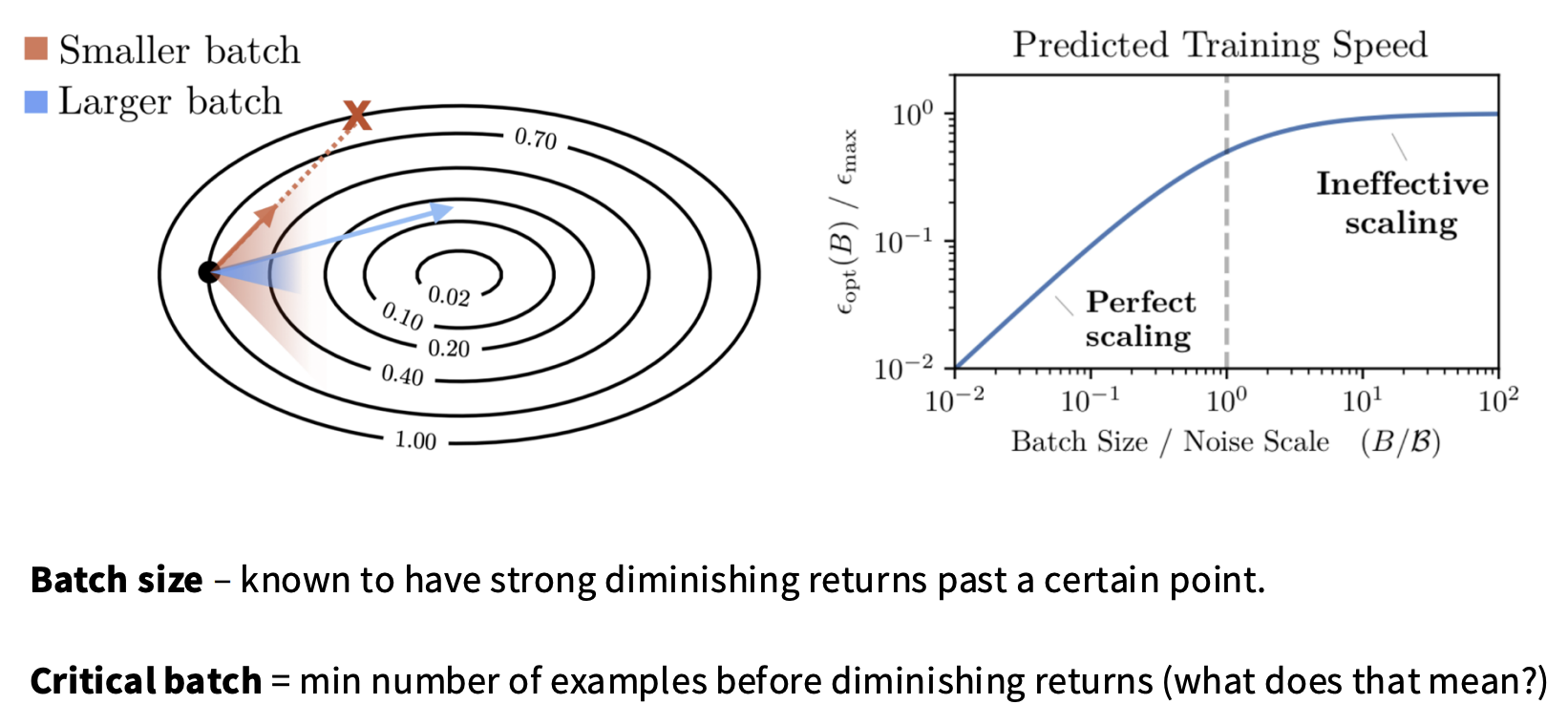
假设critical batch size对应的是点A,在点A之前,模型是variance limited,因为batch过小导致每次更新波动方差很大;在点A之后,模型是bias limited,意味着模型已经可以找到局部最优点,但因为梯度下降没有global view,所以和全局最优始终有bias term存在。
具体参考论文:https://arxiv.org/pdf/1812.06162
从scaling law的角度说,想要loss越低,需要的critical batch size越大:
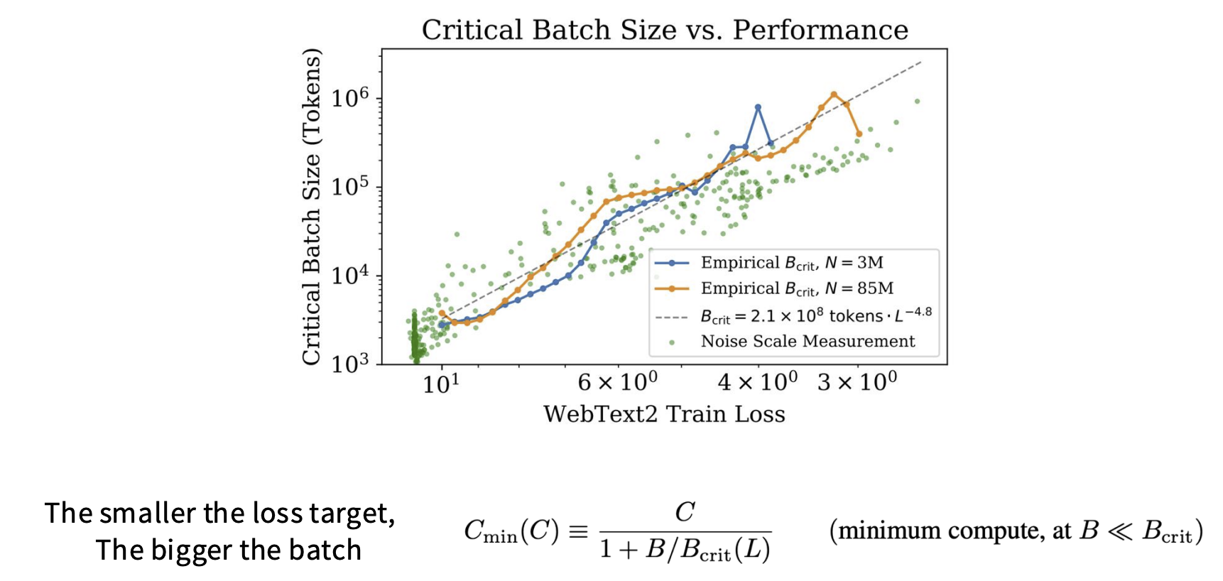
可以这样理解:想要达到的loss越低,越要控制梯度噪声(variance)的影响,所以需要更大的BS,让梯度在正确的极值方向上。
- LR
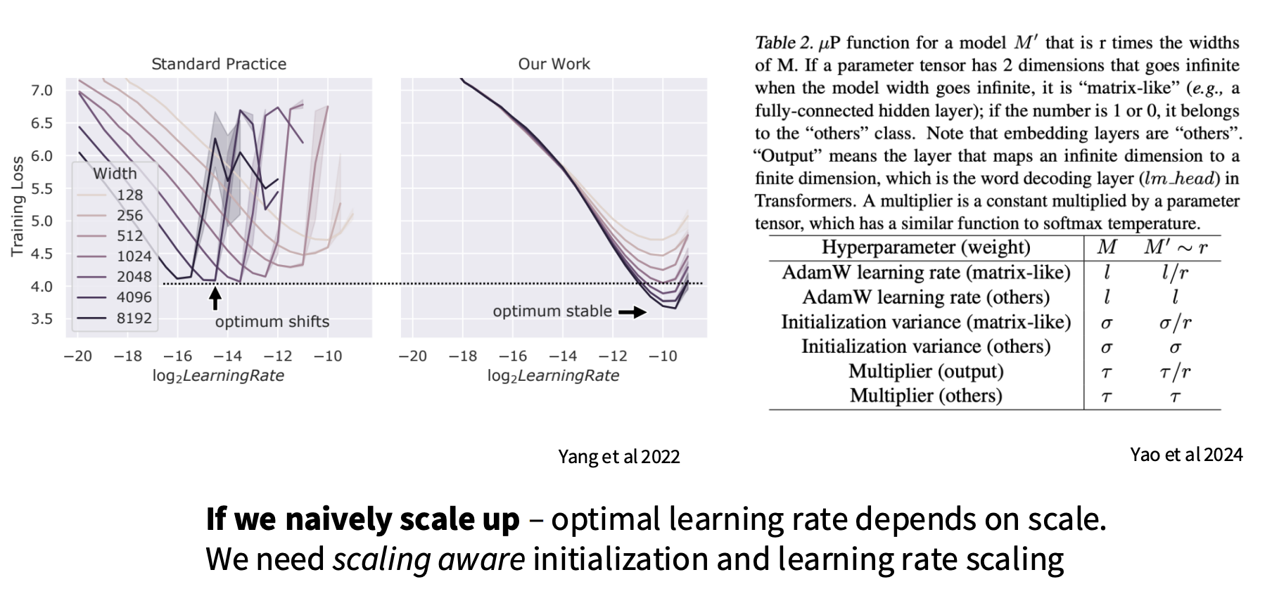
两种调整LR的方法:
- 找到最好的LR,然后通过改变模型initialization size/step size…,避免每次scale都要调整LR,如右侧图所示,这种方法被称为$\mu p$;
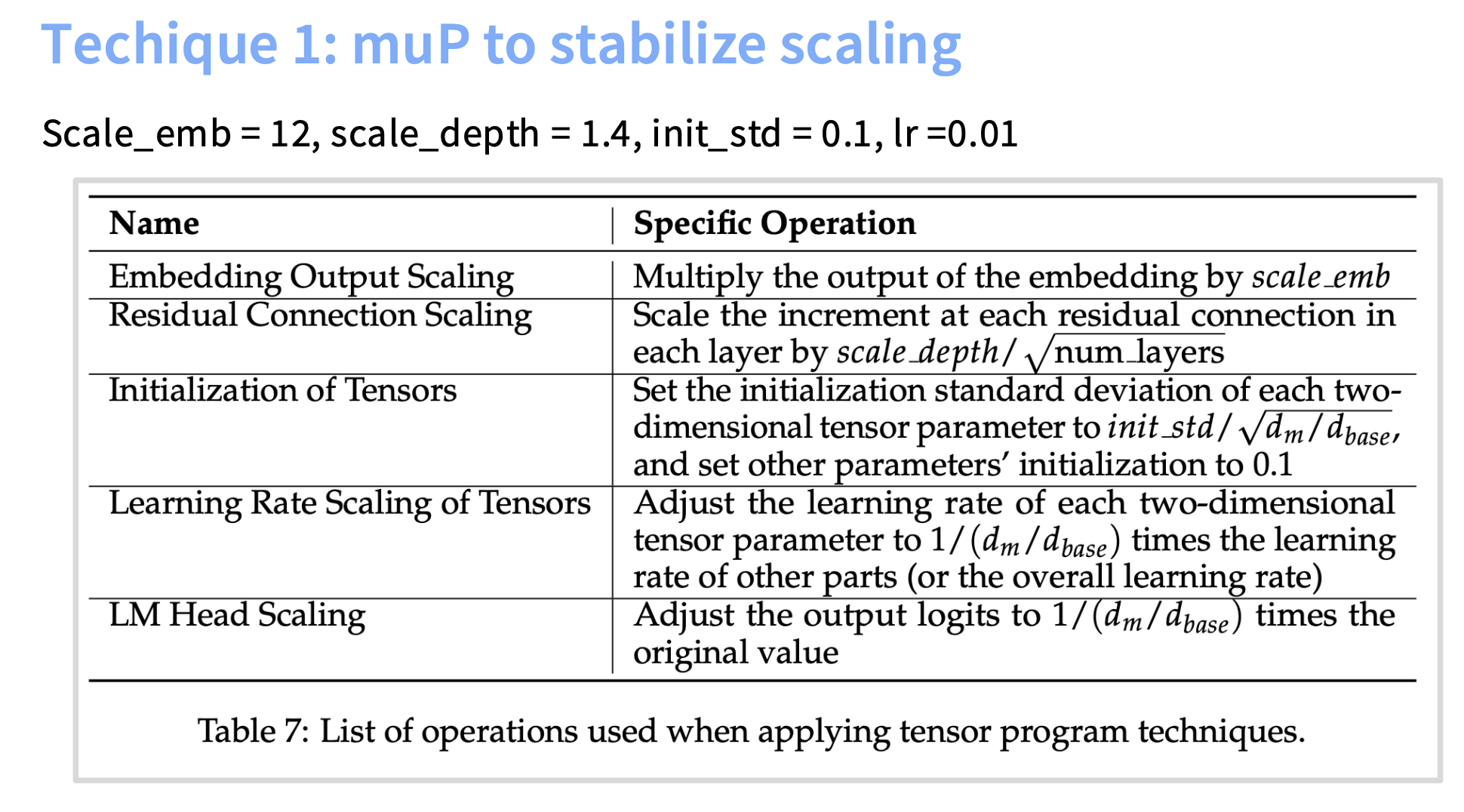
- 根据不同参数量拟合出的曲线,预测当前需要的最好的LR,最佳LR会随着width而改变;如左侧图所示,这是传统的scaling方法;
此外,近两年主流LLM都采用cosine decay的学习率策略,但它有个关键问题,就是对续训很不友好。早在Chinchilla的工作中就提到,cosine策略的衰减周期需要与训练步数一致,过短或过长都不会收敛到当前的局部最优:
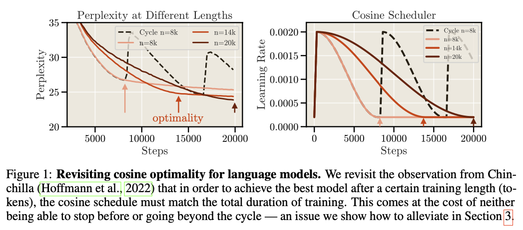
所以不能从一个预期训练10K step的模型上直接拿出5k step的ckpt续训一个6K step的模型。而MiNiCPM的WSD解决了这个问题,即快速warmup后,一大段时间内使用固定学习率,在最后快速衰减到小的学习率。如下图:
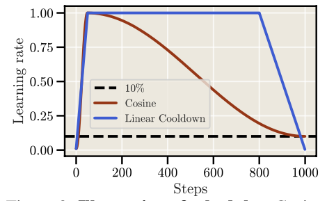
这个策略的核心意义在于让训练中途保存的ckpt尽可能接近真实训练到这个进度的ckpt;在小尺寸模型上的收敛效果很好,甚至快速衰减后还可以超过cosine的表现。WSD策略对续训就更加友好,只要拿到之前固定学习率的ckpt就可以继续训练,节省了很多计算资源,不再需要train from scratch.
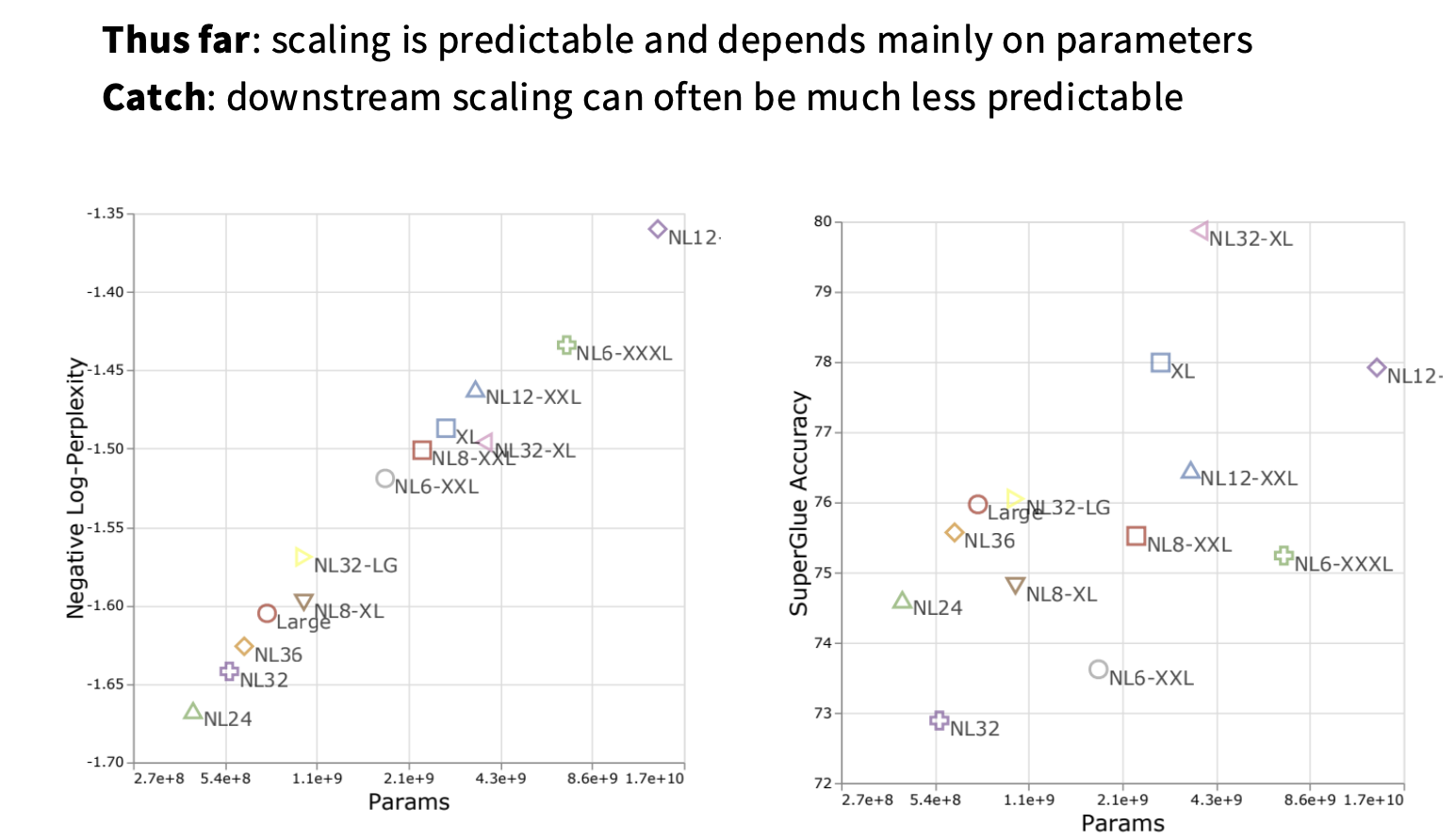
Caution
这里谈论的scaling law基本只对预训练生效:
Joint data-model scaling laws
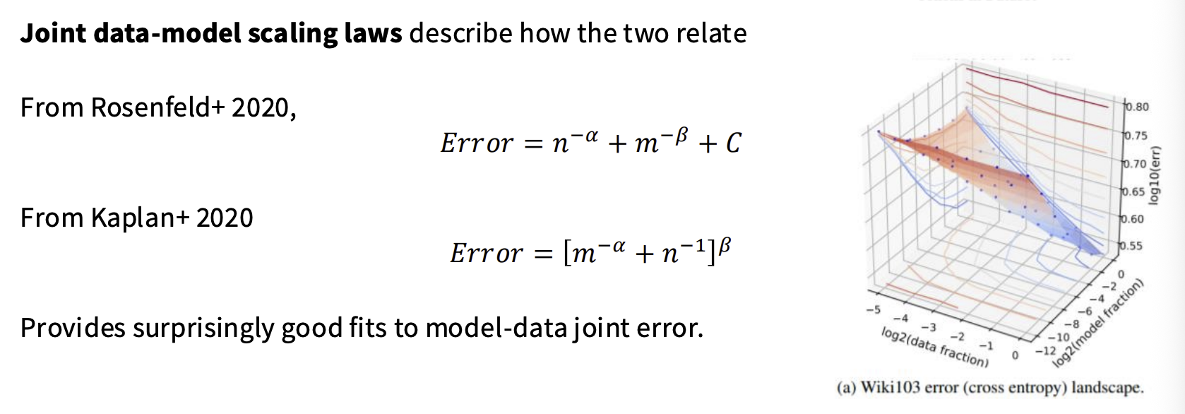
讨论在固定FLOPS下,最佳的token和param的比值。这里只贴一种IsoFLOPS的方法:
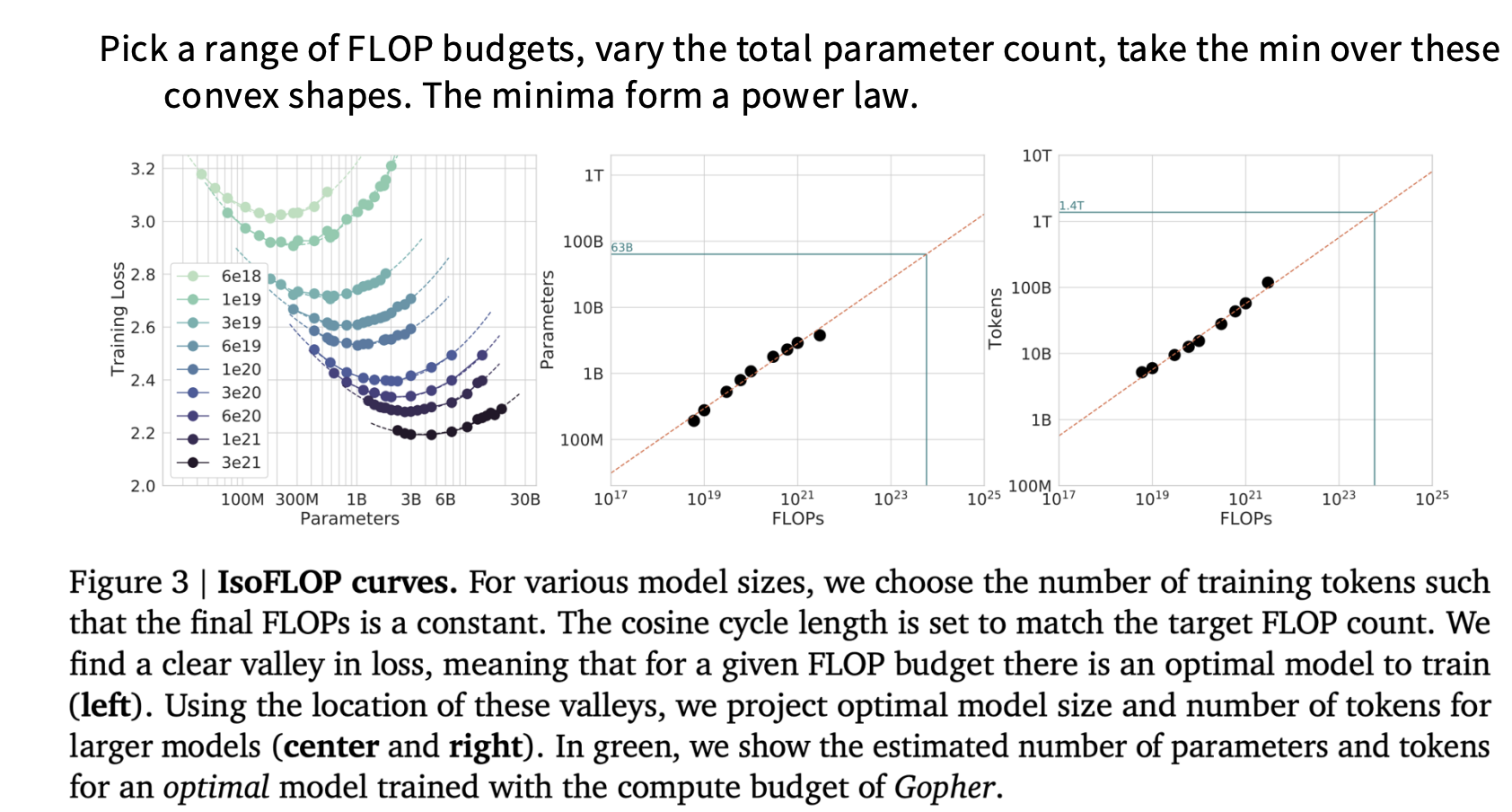
- 相比chinchilla,Kaplan的预测为什么不对?
Kaplan removed last layer param from the count
Warmup at very small compute budgets was too high (模型还没有完全收敛,LR还没有进入到平滑阶段)
- token/param的取值
在Chinchilla的原始论文中,设定为20t/p,但这个结果只是基于优化训练cost(FLOPS)的,随着推理需求的增加,我们应该做overtrain,即耗费更多一次性的训练成本,来优化推理成本(这需要训练更多tokens,过多的param反而会提升推理成本),所以当前token/param在Llama3中就被提升到了215,Mistral是110.
基于这种data-model joint scaling laws prediction, 以及WSD的学习率下降方法,可以用消耗较少资源的方法,得到$D/N$的最优解。在MiNiCPM中,对于每一组不同参数量($N$)的模型,可以用WSD训练一个有较多tokens($D$)的模型,然后在其训练过程中的LR stable phase保存多个不同token量级的ckpt,以及其对应的loss,并绘制出如上方所示的曲线图,得到在这个模型中最优的数据/参数配比。
muon
TODO: 参考 https://kexue.fm/archives/10592。
可以简单理解成做了一个一阶动量的正交化:将奇异值压到相近尺度,抑制大方向并增强其他有效方向。
来自苏神:
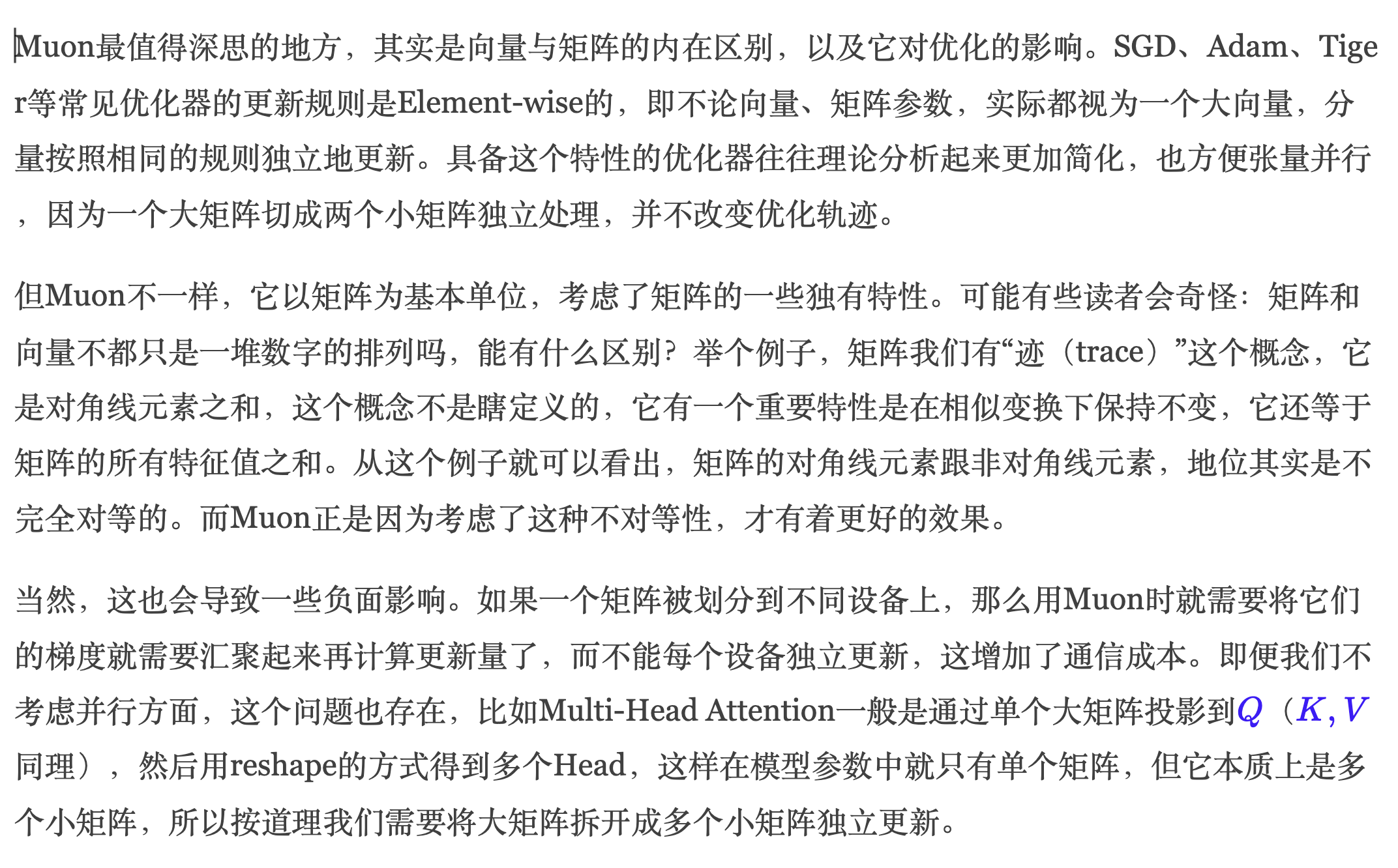
具体而言,使用muon优化器的梯度下降利用了2范数来度量矩阵不同元素的差异。
muP
实在是不想学了。
Inference
KV cache
参考从矩阵运算的角度理解KV Cache。注意是一个sequence(B维度)一个cache.
Inference Workload
Fast metrics:
- Time-to-first-token (TTFT): how long user waits before any generation happens (for interactive applications), is a function of prefill time
- Latency (seconds/token): how fast tokens appear for one query (for interactive applications)
- Throughput (tokens/second): how fast tokens appear for many queries (for batch processing)
arithmetic intensity of inference
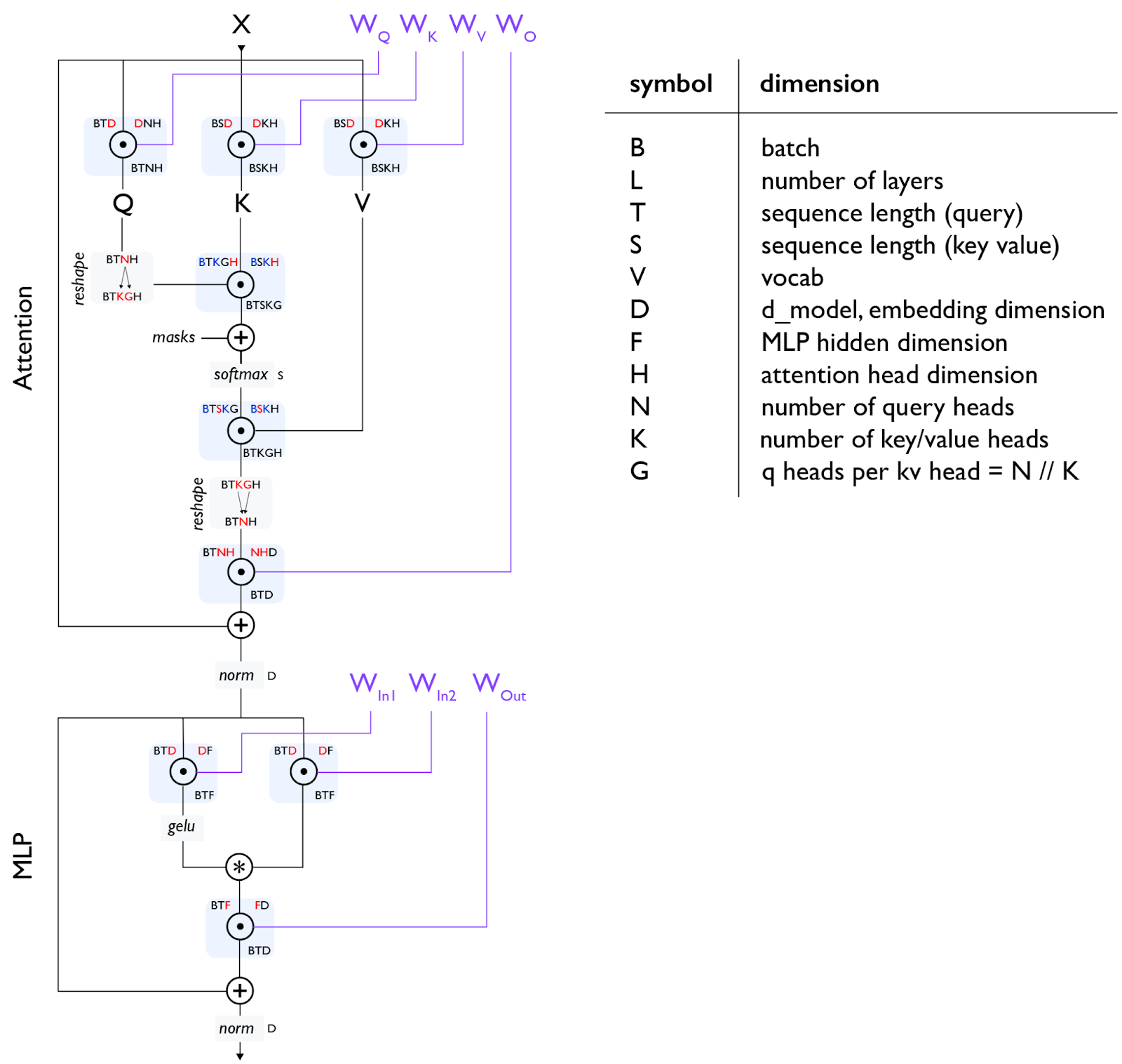
假设$S$是prefill阶段处理的token数量,$T$是生成的token数量(decode/generation阶段)。在prefill阶段,$T=S$,在decode阶段,$T=1$.
Assume that B*T is much smaller than D and F:
$$D=cBT$$ $$F=cBT$$ $$c=\inf$$
- MLP layers
arithmetic intensity = B*T
在decode阶段,B代表并发的requests数量 (所以需要更多的concurrent requests),对于交互应用不可预测。
- Attention layers
prefill: S/2
Decode: < 1 (memory-bound)
throughput and latency
def compute_transformer_performance_stats(config) -> TransformerPerformanceStats:
    """Compute various performance stats for the Transformer given `config`."""
    # Number of parameters in the Transformer
    num_params = 2*V*D + D*F*3*L + (2*D*N*H + 2*D*K*H)*L
    # How much memory the parameters take
    parameter_size = 2*num_params  # 2 for bf16 (training requires a larger multiple)

    # How much the KV cache takes per sequence (S tokens, K heads, H head dim, L layers)
    kv_cache_size_per_seq = S * (K*H) * L * 2 * 2  # 2 for key + value, 2 for bf16
    # Total memory usage
    memory = B * kv_cache_size_per_seq + parameter_size
    # *Latency* is determined by memory IO (read all parameters and KV cache for each step)
    latency = memory / memory_bandwidth
    # *Throughput* is the inverse of latency, but we're generating B tokens in parallel
    throughput = B / latency
    # Substitute config
    num_params = num_params.subs(config).simplify()
    memory = memory.subs(config).simplify()
    latency = latency.subs(config).simplify()
    throughput = throughput.subs(config).simplify()
    return TransformerPerformanceStats(num_params, memory, latency, throughput)
Tradeoff between latency and throughput:
Smaller batch sizes yield better latency but worse throughput
Larger batch sizes yield better throughput but worse latency
在prefill阶段,需要小一些的BS,目的是让TTFT更快;在decode阶段,需要更大的BS,目的是让系统整体的throughput更高。
Make kv inference faster
第一种方法是减小kv cache size.
reduce kv cache size
- MHA, MQA, GQA
- MLA
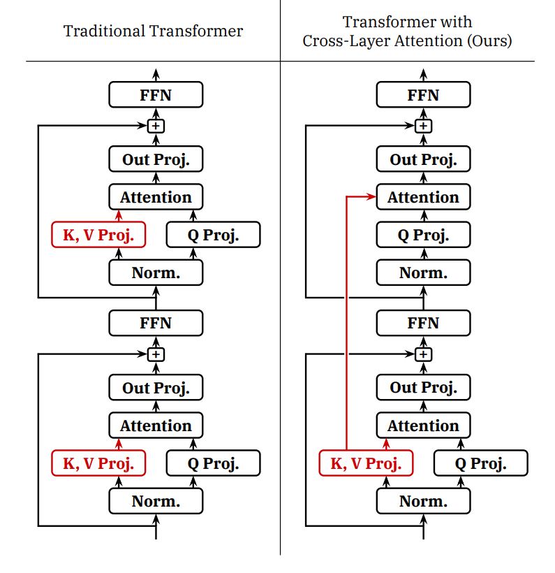
- Cross-layer attention (CLA)
- Local (slidng window) attention
- DeepSeek v4 attention
CSA/DSA/HCA…
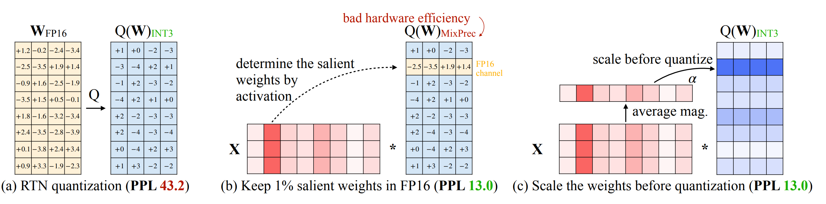
Quantization
- Activation-aware quantization (AWQ)
- Post-training quantization (PTQ)

model pruning
rip out parts of an expensive model to make it cheaper, and then fix it up.
Algorithm:

1. Identify important {layer, head, hidden dimension} on a small calibration dataset (1024 samples)

2. Remove unimportant layers to get a smaller model

3. Distill the original model into pruned model
Speculative sampling
相比上述方法,这种方法是lossless的。核心在优化decode阶段:
利用一个高效的,模型结构较小的近似模型$M_p$生成候选tokens,然后通过目标模型$M_q$验证候选token的合理性,对于合理的token,直接加入当前的输入前缀中,否则从被拒绝的第一个token x开始,往后的所有token都会在被调整后的分布$p'(x)$中做新一轮的投机解码。
由于这个性质,如果每个token被接受的概率是$\alpha$,那将最后加入前缀的数量$n$拆成多个是否存活的随机变量$I_i$,1表示被接受,0表示被拒绝,则:
$$n=I_1+I_2+...+I_k$$对两边同时取期望,又:
$$E(I_i)=1\times P(I_i=1)+0\times P(I_i=0)$$,且$P(I_i=1)=\alpha^i$,
所以是一个等比数列求和:
$$E(n)=\frac{1-\alpha^{k+1}}{1-\alpha}$$
这种方法的优势在于:
- draft model计算开销很小,生成同样数量的token相比标准模型更快;标准模型只需要承担验证的责任;
- 标注新模型可以并行验证多个候选token;由于草稿模型和目标模型分布近似,所以大部分token都被接受,导致开销显著降低;
参考文章:

Continuous batching

解决面对动态workloads的挑战:
最早在orca中被提出:https://www.usenix.org/system/files/osdi22-yu.pdf
下边两张图很好的展示了continuous batching相比传统的static batching带来的收益,TTFT和资源释放时间都被优化:
Selective batching
由于每次attention要处理的是一个$BST$的tensor,所以对于序列长度不同的请求,要做padding,从而导致计算浪费。
- 对attention layer,对请求按照序列长度分组;
- 对MLP layer,将所有序列合并成一个大tensor:[3,H],[9,H] –> [12,H]
Page Attention
先前的系统有两个问题:

- Internal fragmentation:申请过多空间,但实际上没有用到那么多token
- External fragmentation:需要额外申请大段空间,但是在先前申请的连续大块显存中已经找不到那么大的位置,只能在别的位置重新开辟
这本质上是因为CUDA自带的virtual addr机制不感知推理系统,比如无法根据序列长度等信息来决定虚拟地址分配,同时分配粒度又很粗(KB级别)。
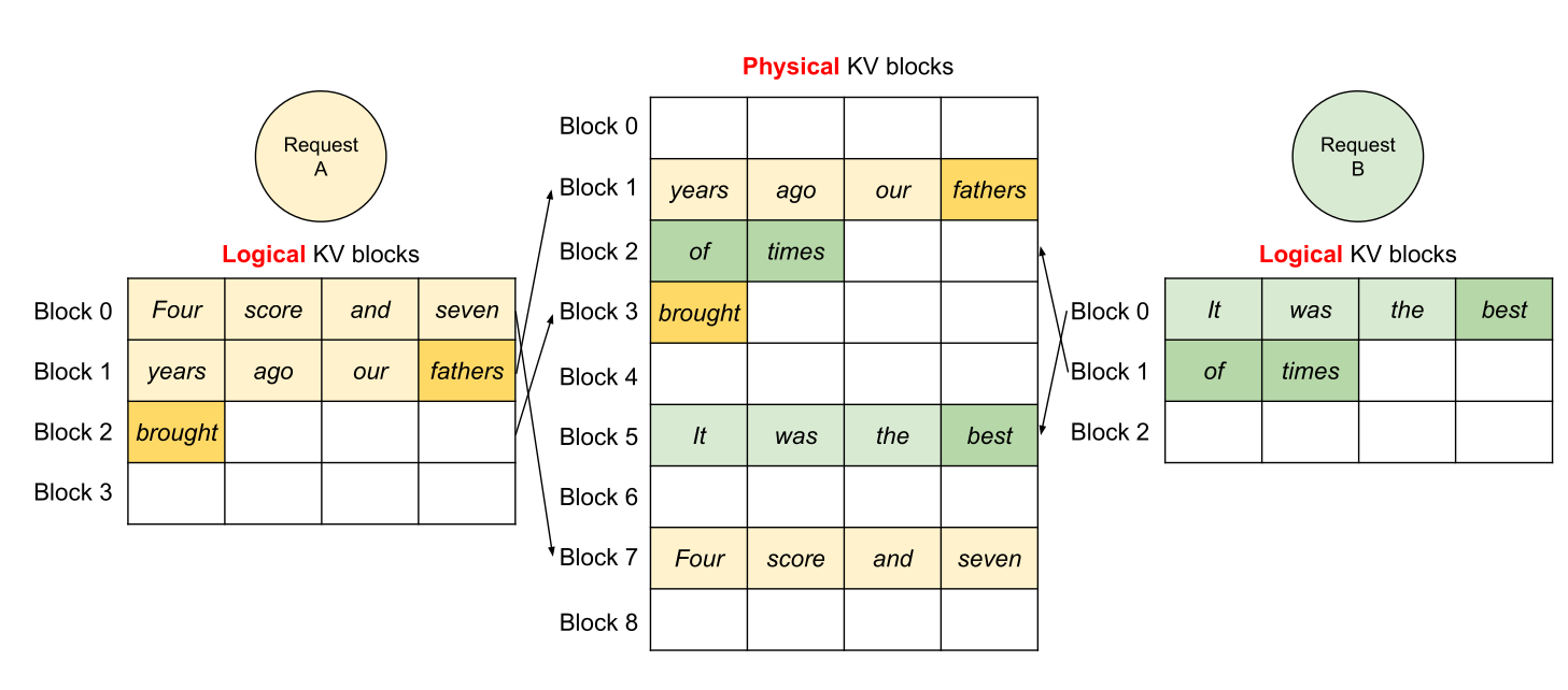
在Page attention中,是将同一个sequence的KV cache分成不连续的blocks,优势在于:
- 更加细粒度的地址分配+感知序列信息,可以缓解先前的碎片问题;
- 多个请求(比如
system prompt)可以共享底层存储;(这里的思路类似OS从虚拟地址到物理地址的映射)
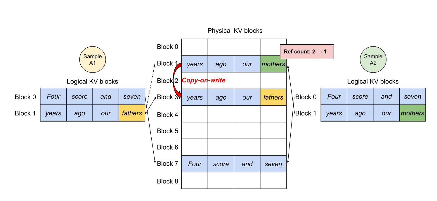
- 可以共享prefixes,使用COW的方法(因为不同请求要更改同一个block,所以必须复制一份):
Evaluation
- Perplexity
困惑度越低,模型性能越好
Data
没做笔记。这部分主要讲预训练使用的数据集。
Mid/Post-Training
在预训练之后,还要让模型学会:当用户以问题形式询问时,应该如何利用已有知识给出合适回答。
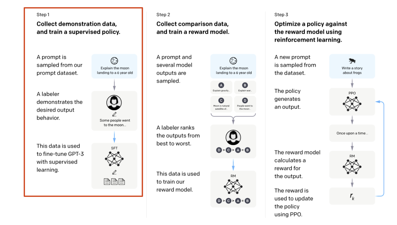
基本流程是SFT+RLHF。
SFT
Datasets
SFT的数据经历了一些迭代:从一开始的大量数据集中抽取的NLP格式的对话数据集,变成人类对话模式,并且添加了更多细节的数据集;再到侧重于工具使用,以及agent友好的数据集:
- “Chattiness” – FLAN is (usually) valid data, but people don’t want to talk to a NLP benchmark. Later datasets move towards longer, more detailed responses
- Detail – OASST goes into much more detail about various factual pieces of knowledge. As we will see, this can be both a pro and a con.
- Tool use – SFT in the last year or two has also been shifting much more towards tool/use, agentic downstream applications.
knowledge extraction and alignment
一个例子是在每个回答的最后都贴一段reference(tail knowledge),但是这些ref未必在原有的(模型在预训练阶段已经见过的)数据集中。
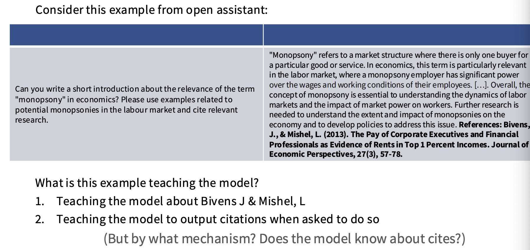
这种让模型在SFT阶段学习它未知的信息的行为,容易让模型产生幻觉, 比如右侧的train unknown曲线,并没有像train known曲线一样快速上升(因为模型本身就具备这些知识),但后来也达到了一样的高度,但模型知识学习到了:“每次输出回答,我都要生成一个看起来像reference的东西”。
John Schulman认为这也是需要RL的原因之一,因为RL提供了学习知识边界的正确目标形式。
safety
其实不仅仅是safety,SFT阶段只要少量的样本就可以产生很大的影响。
Mid-training
在SFT之前,pre-training的LR decay阶段,会遭保留部分通用预训练数据的基础上,提高高质量、专业化数据的比例(这部分数据没有出现在pre-train stable LR的原因是因为token不够),从而将预训练过程拆分成pretrain+mid-training的two-phase training:
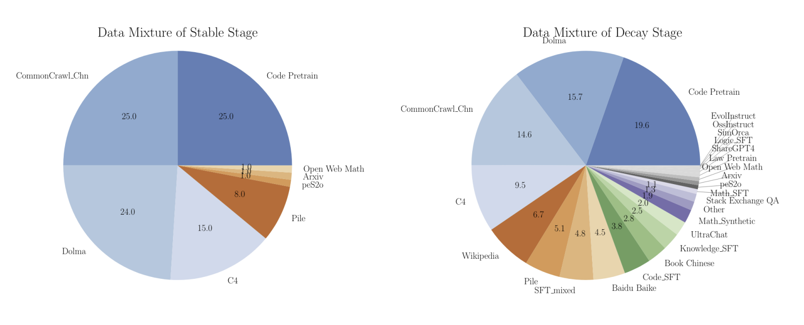
RLHF/RLVR
与在预训练以及SFT阶段拟合模型分布$q(y|x)$贴近目标分布$p(y|x)$不同,RLHF要找到一个$q(y|x)$来最大化reward $R(y,x)$. 这样做的好处是让模型自己search over reasoning trajectories,而不是类似SFT那种强制制定标准答案的方法(从告诉你应该输出什么,到告诉你输出结果好不好),这能充分激发模型的reasoning能力。
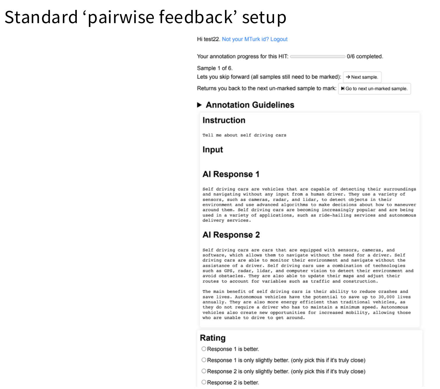
现在常使用model-based annotations来生成/增强后训练数据,因为人力成本太贵而且耗时。
RLHF优化的目标函数$J(\theta)$为$E(R(x,y))-\beta D_{KL}(\pi_\theta||\pi_{SFT})$;这表明:
- 提高 reward 高的回答概率;
- 同时不让优化目标偏离SFT本身的分布太多;
PPO
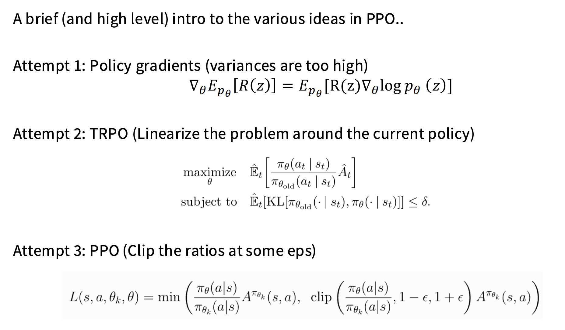
从on-policy到off-policy(采样一次,过多次optimization step),又从实现较为复杂的TRPO进化到了PPO。当然PPO也可以online的做,那样它的$\frac{\pi_\theta}{\pi_{old}}$的比值将永远是1,意味着clip实际没有作用。
- Policy Gradients公式的来源:
为了解决采样过程(即从分布$p_0$中采样$z$,并生成reward $R(z)$)本身不可微的问题,等式右侧的log probability可微,所以在梯度下降时,通过右侧等式告诉模型对于高reward的回答($R(z)>0$)增大它的概率,对于低reward($R(z)<0$)的回答,降低它的概率。
$$E_{p_\theta}[R(z)]=\sum_{z}p_\theta(z)R(z)$$ $$\nabla_\theta E_{p_\theta}[R(z)]=\nabla_\theta\sum_{z}p_\theta(z)R(z)=\sum_{z}\nabla_\theta p_\theta(z)R(z)$$又 $R(z)$与参数无关,故:
上式等价于
$$\sum_zR(z)\nabla_\theta p_\theta(z)$$引入log trick,即通过log函数的求导公式变换得到:
$$\nabla_\theta p_\theta(z)=p_\theta(z)\nabla_\theta \log p_\theta(z)$$代入上式得到:
$$\nabla_\theta E_{p_\theta}[R(z)])=E{p_\theta}[R(z)\nabla_\theta \log p_\theta(z)]$$
- 在TRPO和PPO中,$\frac{\pi_\theta}{{\pi_{old}}}$作为重要性采样比率(
importance sampling ratio),也就是现在这个策略有多想做这个动作->相比采样数据时的旧策略变化了多少;TRPO和PPO本质上都是在控制优化策略不偏离SFT分布太远,只是PPO采用了工程上更容易实现的手段。其中的$A_t$定义为$A_t=Q(s,t)-V_t$,其中$Q$为执行action后的未来总收益,$V$为value function或者说critic model衡量的当前状态平均收益。
DPO
- 不再训练奖励模型,直接使用人类标注的偏好数据,一步到位训练对齐模型
- 不再使用强化学习的方法,通过数学推理,将原始的偏好对齐优化目标步步简化,最后通过类似于sft的方式,用更简化的步骤训练出对齐模型
具体参考:https://zhuanlan.zhihu.com/p/721073733
上文中的分析已经非常详尽了,核心目的是让优化目标中不出现$R(z)$,也就是找到一种方法,使用$\pi(y|x)$来表示$R(z)$,通过将原始的优化目标的分子分母全部利用配分函数(partition function)表示为概率分布的形式,就可以利用优化KL散度的目标来优化模型:KL散度是相对熵,在两分布最接近时最小,从而模型$\pi$有显式解:
这也就是我们找到的奖励函数与策略分布之间的关系,利用该等式,结合Bradley-Terry模型或者Plackett-Luce模型对有优化目标建模并替代其中的奖励函数部分,即可拿到直接优化对齐模型的loss function。但这也是DPO没有被广泛应用的一个原因,即DPO需要这种pairwise的回答输出格式,但并非所有问题都具备这种结构,比如一些数学问题,所以PPO还是更普遍的RLHF方法。
RLHF存在over-optimization的问题,如果训练数据过多,容易对奖励模型过拟合;因为这和优化alphaGO等问题不一样,我们不是在像alphaGO一样,确切的在训练模型实际被使用的场景。
GRPO
相比PPO,GPRO将value function拿掉,将平均收益的衡量变成用当前策略采样N组的平均收益。
- GRPO效果问题:
从最基本的policy gradient出发,对reward function减去任何state-dependent term都可以成立:
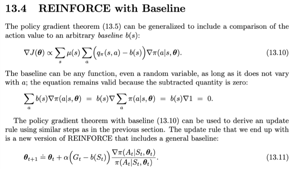
但GRPO恰恰多除以了一个标准差:
$$A_i=\frac{r_i-mean[r_1,r_2, ..., r_G]}{std[r_1,r_2, ..., r_G]}$$这意味着在采样标准差很小时,对效果的影响会比较大,比如问题很简单或者很难,每次正确率都是100%或者0%,这种情况其实是我们不想要的。
此外,当前主流实现还会除上一个采样回答的序列长度(length normalization):
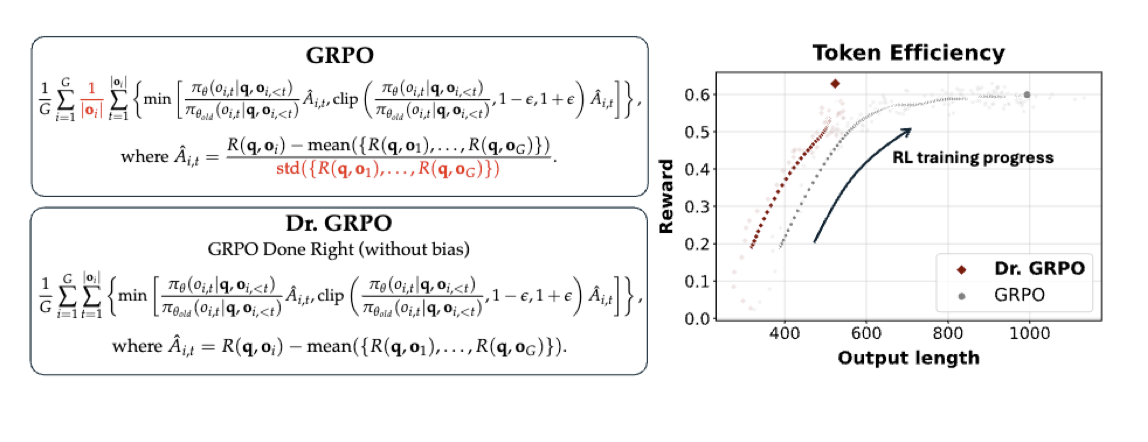
因为总体上希望让奖励值更高,所以对于positive advantages,相比于长回答,反而会激励更短的回答,对于negative advantages,会激励更长的响应。
关于课程后续的几个模型后训练部分的分析内容,有机会会列在单独的blog中做整个report的分析。
Alignment - MultiModallity
最终目标:Omni Model
- Input any combination of modalities (understanding)
- Output any combination of modalities (generation)
Vision Encoder
CLIP
CLIP (Contrastive Language-Image Pretraining)
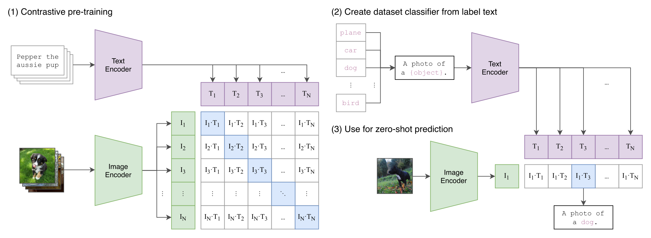
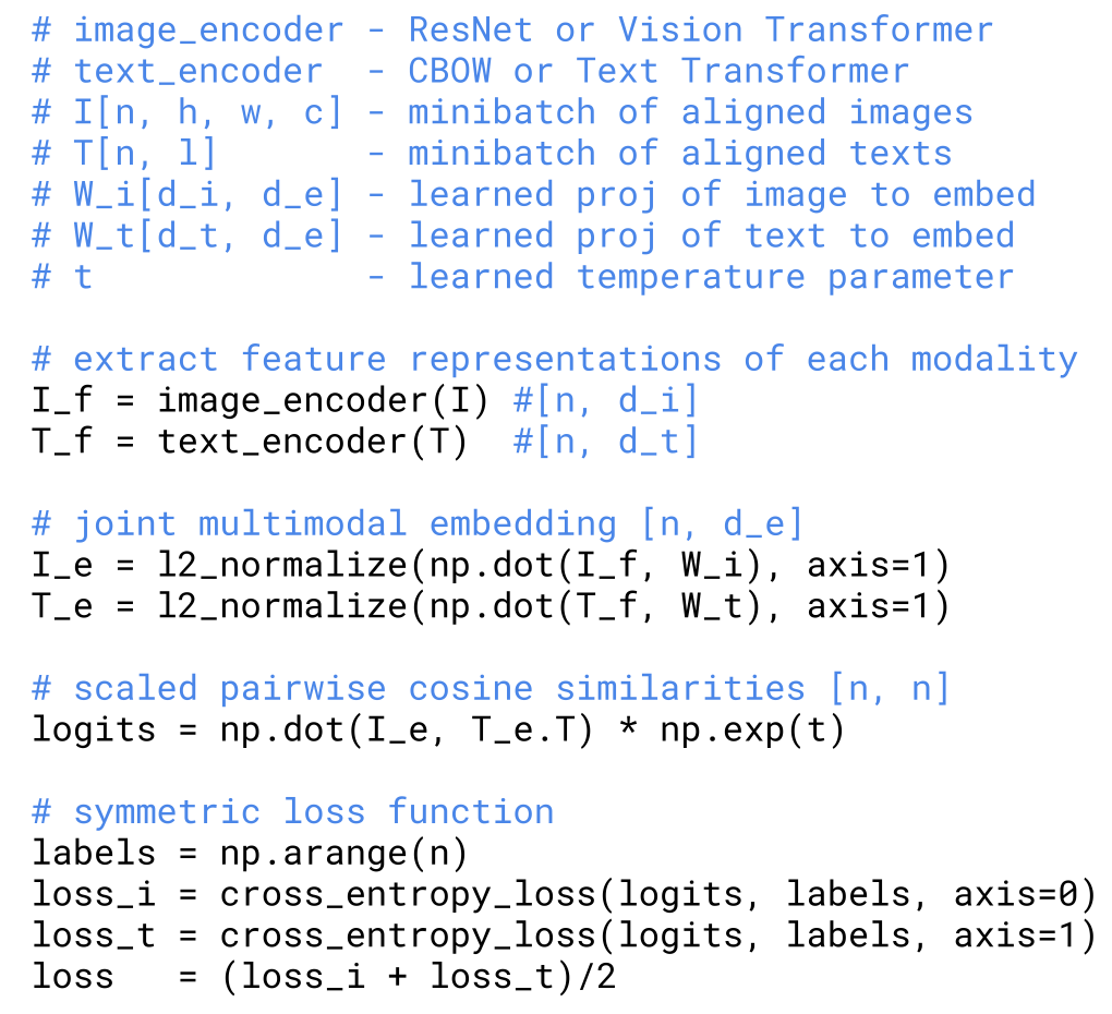
输入batch $(I_1, T_1), (I_2,T_2), ..., (I_n, T_n)$;
经过两个encoder和投影+归一化之后,得到 $u_i\in\mathbb R^d,v_j\in\mathbb R^d$,并且$\|u_i\|_2=\|v_j\|_2=1$。所以上面点积构造的就是一个相似度矩阵,其中$s_{ij}=\alpha u_i^Tv_j$,其中$\alpha$是可学习的logit scale:
$$S= \begin{bmatrix} s_{11}&s_{12}&\cdots&s_{1n}\\ s_{21}&s_{22}&\cdots&s_{2n}\\ \vdots&\vdots&\ddots&\vdots\\ s_{n1}&s_{n2}&\cdots&s_{nn} \end{bmatrix}$$对image2text loss和text2image loss,只需要看一种情况即可,以image2text loss为例:
对每行做softmax:
$$p_{ij}=P(T_j|I_i)=\frac{e^{s_{ij}}}{\sum^n_{k=1}e^{s_{ik}}}$$根据交叉熵定义:
$$\ell_i = -\sum_{j=1}^{n}y_{ij}\log p_{ij}$$由于one-hot label在一行内只有一个位置是1,故:
$$\ell_i^{I\to T} = -\log p_{ii}$$代入并整合:
$$\ell_i^{I\to T} = -s_{ii} + \log\sum_{j=1}^{n}e^{s_{ij}}$$整个batch的image2text loss为:
对第$i$行的某个$s_{ij}$求导:
- 对于对角线位置(i==j)
则$s_{ii}$在梯度下降后变大。
- 对于非对角线位置(i!=j)
则$s_{ij}$在梯度下降后变小。
text2image loss同理,所以结论是:
- 对每一张图片,更倾向于和其
aligned的text; - 对每段text,更倾向于和其
aligned的图片;
当目标标签是对角矩阵、loss 是 softmax cross-entropy 时,对相似度矩阵的负梯度方向必然提高对角项、降低非对角项.
更一般的规律是:预测概率矩阵$P$会被推动着接近目标矩阵 $Y$。
CLIP 里恰好:
$$ Y=I_n $$所以看起来是“朝对角线前进”。
ViT
Vision Encoder:
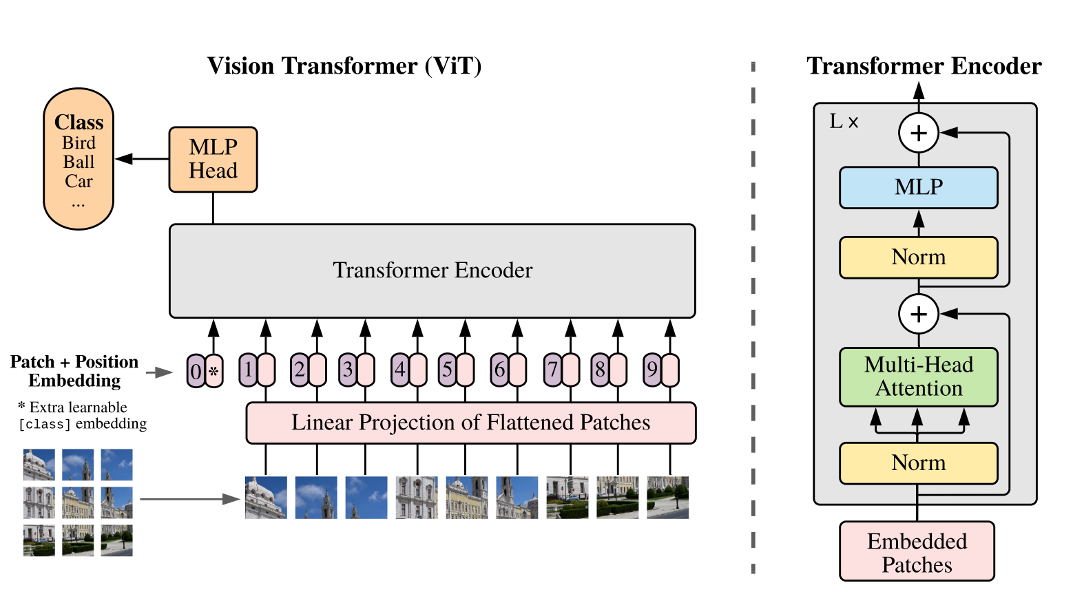
- Attention pooling: do QKV with query = global average of activations
上述CLIP方法存在的问题:需要比较大的BS(因为样例本身包含了label信息),同时softmax操作是对整个batch做的,没办法很好的并行。
siglip
将CLIP的多分类问题转化为一个二分类问题,即判定$(T_i,I_j)$是否是对齐的配对。
之前的多分类问题来源于多种label的存在,所以使用了softmax,这里将label $y_{ij}$转化为只有$(-1,1)$矩阵的形式。同时建立损失函数为:
$$\ell_{ij} = -\log\sigma(y_{ij}s_{ij})$$其中$\sigma$为log-sigmoid函数,这里的计算是逐元素乘法。
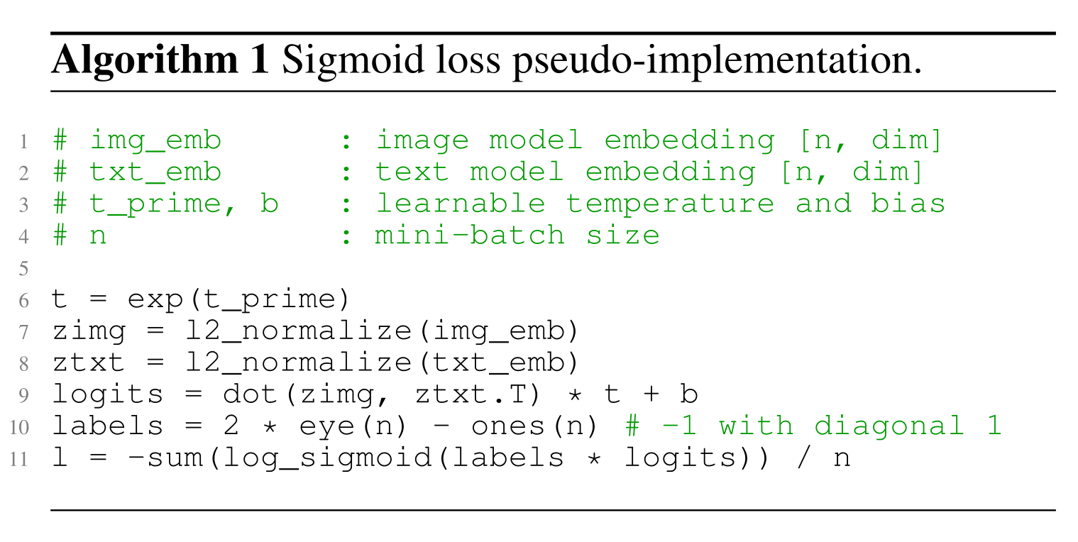
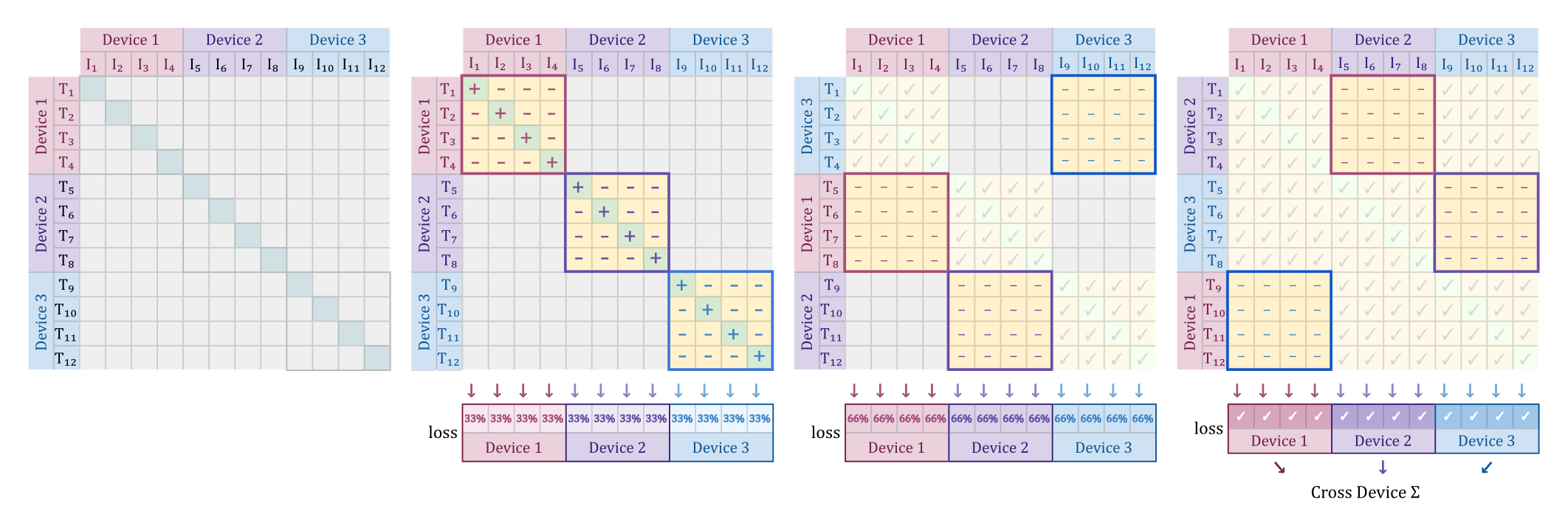
siglip的优势在于较快的训练速度,因为其不和BS绑定,loss function的计算可以在不同设备上并行执行:
Inject image encodings into LLMs
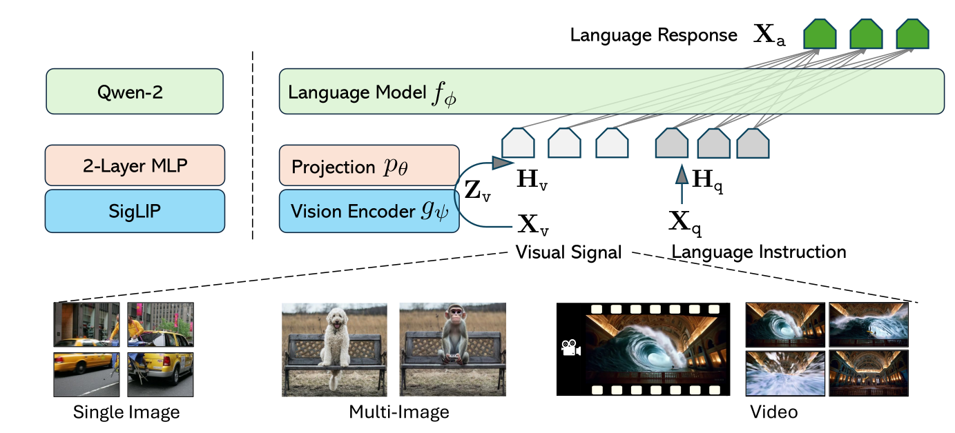
关于qwen系列多模态的细节介绍,也会放到单独的blog里讲。
Omni model
与VLM不同的是:VLM往往需要多模态输入+text输出,但是对于omni model,更希望做到多模态输入+多模态输出。所以需要将图片/声音等也组织称文本一样,离散的、可以逐token预测的vocabulary。
使用CLIP/SIGLIP类似的将图片直接转化成连续向量的方法无法让LLM生成多模态内容,因为此时的输出向量是任意的$d$维实数向量,并非在一个固定的词表里查找得到的。
所以一个自然的思路是将多模态输入也tokenization。
VQ-VAE
一种思路是VQ-VAE.
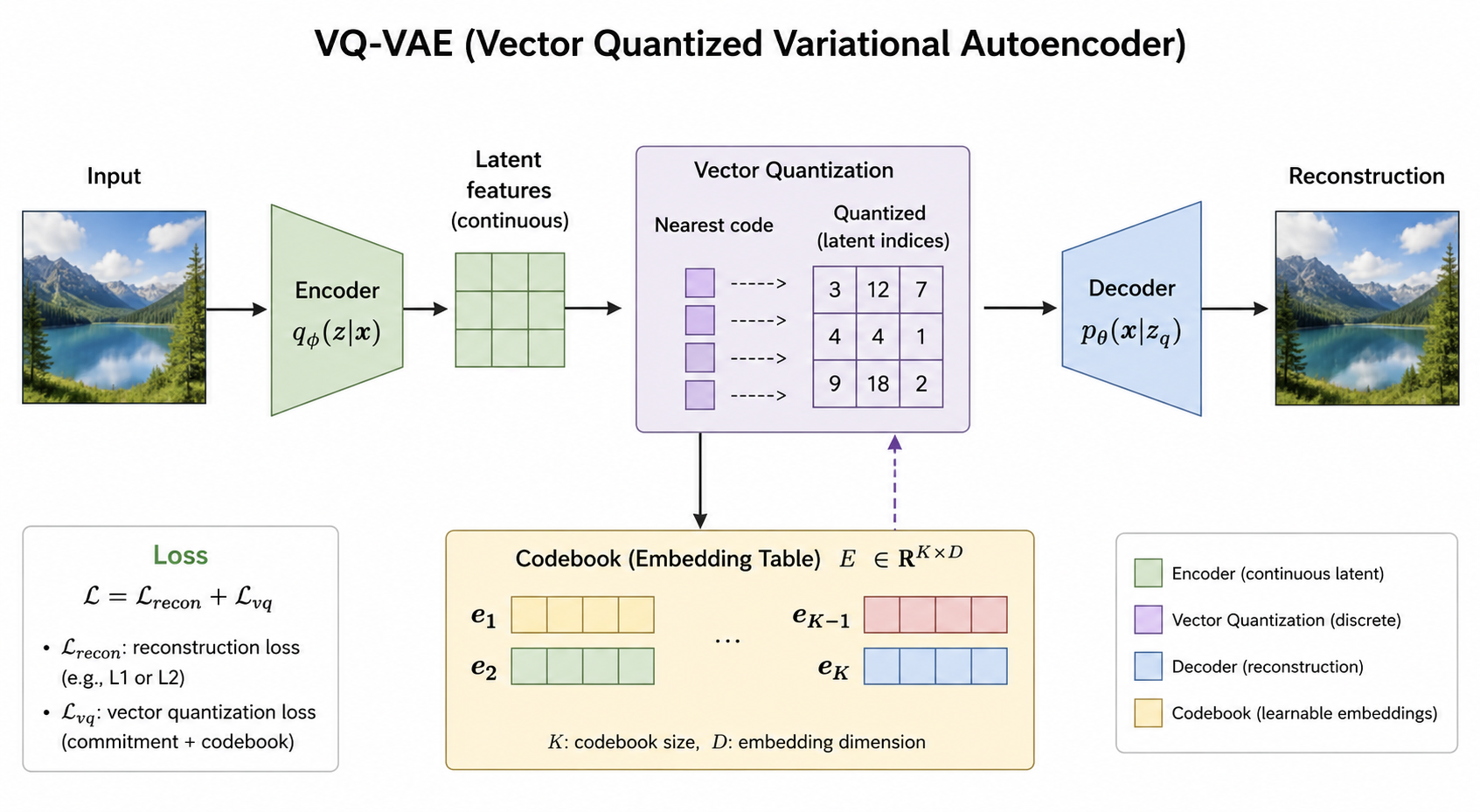
Encodes 512 x 512 image into 1024 tokens (codebook of size 8192)
Train a new BPE tokenizer